Position Navigation and Timing (PNT)

Est. read time: 18 minutes | Last updated: July 17, 2026 by John Gentile

Contents

GPS
Other Methods of PNT

import numpy as np
from scipy import signal
import matplotlib.pyplot as plt
from rfproto import plot

import datetime
import dateutil.parser

GPS

Frequency Domain Acquisition

# Parameters for GPS L1 C/A signal
code_length = 1023                    # Length of C/A Gold code / PRN (chips)
prn_rate    = 1000                    # PRN repitition rate (Hz)
prn_period  = 1.0 / prn_rate          # Time to correlate PRN over (seconds)
chip_rate   = prn_rate * code_length  # C/A code chip rate (Hz)
bit_rate    = 50                      # Navigation data bit rate (bit/sec)
fc_l1       = 1575.42e6               # GPS L1 Center Frequency (Hz)

sps = 2 # Samples/symbol (oversampling rate) of input I/Q data
fs = sps * chip_rate # input sample rate of I/Q file (Hz)
utc_start_time = dateutil.parser.parse("2023-11-03T18:48:00+00:00")

num_seconds = 1
num_samples = int(num_seconds * fs)
# NumPy complex64 type is a complex number data type composed of two single-precision (32-bit) floating-point numbers, 
# one for the real component and one for the imaginary component
iq_in = np.fromfile("./data/nov_3_time_18_48_st_ives-short.fc32", dtype=np.complex64, count=num_samples, offset=0)

# G2 phase selector taps for each SV (1-37) from GPS ICD-200
# Each SV uses two taps from the G2 register to generate its unique C/A code
G2_TAPS: dict[int, tuple[int, int]] = {
    1: (2, 6),
    2: (3, 7),
    3: (4, 8),
    4: (5, 9),
    5: (1, 9),
    6: (2, 10),
    7: (1, 8),
    8: (2, 9),
    9: (3, 10),
    10: (2, 3),
    11: (3, 4),
    12: (5, 6),
    13: (6, 7),
    14: (7, 8),
    15: (8, 9),
    16: (9, 10),
    17: (1, 4),
    18: (2, 5),
    19: (3, 6),
    20: (4, 7),
    21: (5, 8),
    22: (6, 9),
    23: (1, 3),
    24: (4, 6),
    25: (5, 7),
    26: (6, 8),
    27: (7, 9),
    28: (8, 10),
    29: (1, 6),
    30: (2, 7),
    31: (3, 8),
    32: (4, 9),
    33: (5, 10),
    34: (4, 10),
    35: (1, 7),
    36: (2, 8),
    37: (4, 10),
}

def generate_ca_code(sv: int):
    """Generate the GPS C/A (Coarse/Acquisition) code for a given satellite vehicle.

    The C/A code is a 1023-chip Gold code generated from two 10-bit Linear Feedback
    Shift Registers (G1 and G2). Each satellite has a unique code determined by
    different tap selections on the G2 register.

    G1 polynomial: x^10 + x^3 + 1 (taps at 3 and 10)
    G2 polynomial: x^10 + x^9 + x^8 + x^6 + x^3 + x^2 + 1 (taps at 2, 3, 6, 8, 9, 10)

    Reference: https://www.mathworks.com/matlabcentral/fileexchange/14670-gps-c-a-code-generator
    """
    if sv < 1 or sv > 37:
        raise ValueError(f"SV must be in range 1-37, got {sv}")

    # Get tap selections for this SV (convert to 0-indexed)
    tap1, tap2 = G2_TAPS[sv]
    tap1_idx = tap1 - 1
    tap2_idx = tap2 - 1

    # Initialize both registers with all 1s
    g1 = np.ones(10, dtype=np.int8)
    g2 = np.ones(10, dtype=np.int8)

    # Generate the C/A code
    ca_code = np.zeros(code_length, dtype=np.int8)

    for i in range(code_length):
        # Output is G1[9] XOR G2[tap1] XOR G2[tap2]
        g1_out = g1[9]
        g2_out = g2[tap1_idx] ^ g2[tap2_idx]
        ca_code[i] = g1_out ^ g2_out

        # Compute feedback bits before shifting
        # G1 feedback: positions 3 and 10 (indices 2 and 9)
        g1_feedback = g1[2] ^ g1[9]

        # G2 feedback: positions 2, 3, 6, 8, 9, 10 (indices 1, 2, 5, 7, 8, 9)
        g2_feedback = g2[1] ^ g2[2] ^ g2[5] ^ g2[7] ^ g2[8] ^ g2[9]

        # Shift registers right and insert feedback at position 0
        g1[1:] = g1[:-1]
        g1[0] = g1_feedback

        g2[1:] = g2[:-1]
        g2[0] = g2_feedback

    ## Convert from {0, 1} to {1, -1} (0 -> 1, 1 -> -1)
    #return 1 - 2 * ca_code
    return (2 * ca_code) - 1

# Precompute freq. domain PRN code for each SV at proper SPS
prn_fft_sv = []
for i in range(1, 38):
    prn_i = generate_ca_code(i)
    # Upsample PRN code to match input rate and convert to complex with a zero imaginary part
    prn_up = np.repeat(prn_i, sps).astype(complex)
    # In frequency domain cross-correlation, one part needs to be conjugated, so do that now
    prn_freq = np.conj(np.fft.fft(prn_up))
    
    prn_fft_sv.append(prn_freq)

# Compute number of samples to cross-correlate against
num_corr = int(fs * prn_period)
assert len(prn_fft_sv[0]) == num_corr

Parallel Code Phase Search (PCPS) Acquisition

First, we show the “traditional” Parallel Code Phase Search (PCPS) approach, which efficiently searches across Doppler offsets and correlates in the frequency domain:

r[n] \circledast x[-n] = \text{IFFT} \bigg\{ \text{FFT}\{r[n]\} (\text{FFT}\{x[n]\})^{*} \bigg\}

This canonical DSSS acquisition method tests each Doppler hypothesis $f_{d} \in [f_{min}, f_{max}]$ in multiple, iterative steps:

Carrier wipe-off input samples: $x[n] = r[n] \cdot e^{-j 2\pi f_{d} n t}$
Forward FFT these samples: $X[k] = \text{FFT}(x[n])$
Frequency domain multiplication (same as convolution in time domain) of samples and FFT’ed matched (complex conjugated) spreading code: $Y[k] = X[k] \cdot PN_{FFT}[k]^{*}$
Inverse FFT $y[n] = \text{IFFT}(Y[k])$
Detect magnitude peak (e.x. CFAR of $$ y[n] ^2$$)

Acquisition is the 2-D search for $(\tau,f_D)$ that maximizes the correlation (the cross-ambiguity function):

R(\tau,f_D)=\sum_{n=0}^{N-1} r[n]\,c[n-\tau]\,e^{-j2\pi f_D n/f_s},\qquad \hat\tau,\hat f_D=\arg\max |R|^2

# Define Doppler shift range to search (in Hz)
doppler_shifts = np.linspace(-5000, 5000, 100)  # -5 kHz to 5 kHz, 100 steps

# Array to store correlation results: [doppler shifts, time delays]
correlation_results = np.zeros((len(doppler_shifts), num_corr))

# TODO: show search via:
#for sv_idx, sv in enumerate(prn_fft_sv):
sv_idx = 31
sv = prn_fft_sv[sv_idx]

for dop_idx, doppler_shift in enumerate(doppler_shifts):
    # Time vector for Doppler adjustment
    t = np.arange(num_corr) / fs
    # Carrier wipeoff: apply Doppler shift with complex exponential (phasor)
    doppler_adjustment = np.exp(-1j * 2 * np.pi * doppler_shift * t)
    adjusted_signal = iq_in[:num_corr] * doppler_adjustment
    
    # Frequency domain cross-correlation
    fft_signal = np.fft.fft(adjusted_signal)
    cross_corr_freq = fft_signal * sv
    cross_corr_time = np.fft.ifft(cross_corr_freq)

    # Store magnitude of correlation
    correlation_results[dop_idx, :] = np.abs(cross_corr_time)

# Normalize correlation results to [0, 1] to make peak stand out
Z = correlation_results / np.max(correlation_results)

# Define axes: convert samples to C/A code chips
x = np.arange(num_corr) / sps  # PRN code phase in chips
y = doppler_shifts / 1000       # Doppler shifts in kHz
X, Y = np.meshgrid(x, y)

# Create figure with larger size for better detail
fig = plt.figure(figsize=(14, 9))
ax = fig.add_subplot(111, projection='3d')

# Plot with jet colormap, fine stride, and shading
surf = ax.plot_surface(
    X, Y, Z,
    cmap='jet',
    rstride=1,
    cstride=4,
    antialiased=True,
    linewidth=0,
    alpha=0.95,
)

ax.set_xlabel('Code Phase (chips)', fontsize=12, labelpad=10)
ax.set_ylabel('Doppler Shift (kHz)', fontsize=12, labelpad=10)
ax.set_zlabel('Normalized Correlation', fontsize=12, labelpad=10)
ax.set_title(f'GPS L1 C/A Acquisition — SV {sv_idx + 1}', fontsize=14, fontweight='bold')

# Viewing angle: elevated and rotated to show the peak clearly
ax.view_init(elev=15, azim=225)

# Tighten z-axis to emphasize the peak
ax.set_zlim(0, 1.15)

# Find peak and annotate
peak_dop_idx, peak_phase_idx = np.unravel_index(np.argmax(correlation_results), correlation_results.shape)
peak_phase_chips = peak_phase_idx / sps
peak_doppler_khz = doppler_shifts[peak_dop_idx] / 1000
peak_mag = correlation_results[peak_dop_idx, peak_phase_idx]

annotation = (
    f"Corr: {peak_mag:.1f}\n"
    f"Phase: {peak_phase_chips:.1f} chips\n"
    f"Doppler: {doppler_shifts[peak_dop_idx]:.1f} Hz"
)
ax.text(
    peak_phase_chips, peak_doppler_khz, 1.12,
    annotation,
    fontsize=8, fontfamily='monospace',
    ha='center', va='bottom',
    bbox=dict(boxstyle='round,pad=0.4', facecolor='white', edgecolor='black', alpha=0.85),
    zorder=10,
)
ax.plot(
    [peak_phase_chips, peak_phase_chips],
    [peak_doppler_khz, peak_doppler_khz],
    [1.0, 1.12],
    color='black', linewidth=1, linestyle='--', zorder=9,
)

fig.colorbar(surf, shrink=0.55, aspect=12, pad=0.1, label='Normalized Correlation')
plt.tight_layout()
plt.show()

png

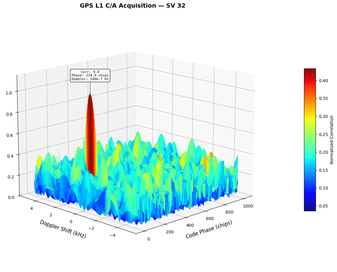
Double-Buffered Joint Frequency and Delay Correlation

Instead of iterating over every doppler bin, performing carrier wipeoff, then performing frequency domain cross-correlation, we can perform joint frequency and delay correlation by:

FFT the received signal once (length N)
Build a Hankel index matrix where each column is the FFT circularly shifted by a different Doppler offset- this is the key trick. A circular shift of $l$ DFT samples in the frequency domain, $X((k-l))_{N}$ , is equivalent to multiplying by a complex exponential (frequency shift) in the time domain, $x(n) * e^{j\frac{2\pi}{N}ln}$ .
Vectorized correlation where we multiply fft(b) * conj(fft_shifted(a)) for all Dopplers simultaneously via matrix operations, then IFFT column-wise.

However it should be seen that, unlike the above traditional method where we can arbitrarily define the Doppler search space (e.g. more or less carrier wipeoff frequency steps), this joint approach has a fixed Doppler bin spacing dictated by the PRN period ( $N$ samples long) of:

\Delta f = f_{s} / N

For coherent correlation, this will almost always equal the PRN rate (1000 Hz in this GPS case). We can calculate coherent integration loss of a given Doppler bin spacing as it’s the same as the DFT (each bin in the DFT is a correlation over the time interval of the sequence to the particular frequency in that bin): when your Doppler hypothesis is offset from truth by $\Delta f$ , the correlation magnitude follows a sinc envelope:

| R(\Delta f)| = | \text{sinc}(\pi \cdot \Delta f \cdot T_{coh})|

Where $T_{coh}$ is the coherent integration time, which for GPS of 1ms gives: | Point | Formula | Doppler Bin Spacing | | —– | ——- | ——————- | | First null | $1/T_{coh}$ | 1000 Hz | | 3 dB point | $~0.44/T_{coh}$ | 440 Hz | | 1 dB loss | $~0.29/T_{coh}$ | 290 Hz |

Essentially longer coherent integration time, and thereby narrower Doppler bins, improves acquisition SNR at the cost of increased search space and computational cost (e.g. acquisition time). Since DSSS processing gain follows $10\cdot \log_{10}(N)$ , we can expect that doubling or halving the coherent integration period results in +3dB and -3dB processing gain, respectively. The tradeoff also needs to factor in Probability of False Alarm (PFA) vs probability of detection.

def fdcorr(a, b, frange=None):
    """Joint frequency and delay correlation using the circular shift property of the DFT.

    Efficiently computes circular cross-correlation between two vectors over all
    possible frequency offsets (Dopplers) by exploiting the fact that a frequency
    shift in time is equivalent to a circular index shift in the frequency domain.
    Instead of looping over each Doppler bin, a Hankel-like index matrix creates
    all Doppler-shifted FFTs simultaneously, enabling a fully vectorized correlation.

    Based on: Dan Boschen, "FDCORR Joint frequency and delay correlation", 2009

    Parameters
    ----------
    a : array_like
        Received signal vector (sampled at fs = 2*pi).
    b : array_like
        Correlation code vector (sampled at fs = 2*pi).
    frange : tuple of (float, float), optional
        Frequency search range as (low, high) in radians, within [-pi, pi].
        Limiting this improves efficiency when Doppler offsets are small
        relative to the Nyquist bandwidth.

    Returns
    -------
    fd_surface : ndarray, shape (N, num_freqs)
        2D correlation surface: rows are delay bins, columns are frequency bins.
    freq_axis : ndarray
        Normalized frequency values (rad/sample) aligned to the frequency axis.
    """
    a = np.asarray(a).ravel()
    b = np.asarray(b).ravel()
    N = max(len(a), len(b))

    fft_a = np.fft.fft(a, N)

    # Frequency axis: centered from -pi to pi (equivalent to fftshift ordering)
    freq_index = np.arange(-np.floor((N - 1) / 2), np.floor(N / 2) + 1, dtype=int)
    freq_axis = freq_index * 2 * np.pi / N

    if frange is not None:
        mask = (freq_axis >= frange[0]) & (freq_axis <= frange[1])
        freq_axis = freq_axis[mask]
        freq_index = freq_index[mask]

    num_freqs = len(freq_index)

    # Build Hankel index matrix: each column is the FFT of 'a' circularly shifted
    # by a different Doppler offset. This is the core trick — a circular shift in
    # the frequency domain corresponds to multiplication by a complex exponential
    # (frequency shift) in the time domain.
    fft_idx = np.arange(N).reshape(-1, 1)   # (N, 1)
    shifts = freq_index.reshape(1, -1)      # (1, num_freqs)
    hankel_idx = (fft_idx + shifts) % N     # (N, num_freqs) circular indices

    fft_dopplers = fft_a[hankel_idx]        # All Doppler-shifted FFTs at once

    # Circular correlation: ifft(fft(b) * conj(fft_shifted(a))) for all Dopplers
    fft_b = np.fft.fft(b, N).reshape(-1, 1)  # (N, 1) broadcast across freq columns
    fd_surface = np.fft.ifft(fft_b * np.conj(fft_dopplers), axis=0)

    return fd_surface, freq_axis


# --- Run joint frequency-delay acquisition for a single SV ---
sv_idx = 31  # SV 32 (0-indexed)
prn_code = generate_ca_code(sv_idx + 1)
prn_up = np.repeat(prn_code, sps).astype(complex)

# Limit Doppler search to +/-5 kHz expressed in normalized frequency (rad/sample)
# Normalized freq = 2*pi * f_hz / fs
max_doppler_hz = 5000
frange_norm = (-2 * np.pi * max_doppler_hz / fs, 2 * np.pi * max_doppler_hz / fs)

fd_surface, freq_axis_norm = fdcorr(iq_in[:num_corr], prn_up, frange=frange_norm)

# Convert axes to physical units
freq_axis_hz = freq_axis_norm * fs / (2 * np.pi)  # Normalized rad/sample -> Hz
delay_chips = np.arange(fd_surface.shape[0]) / sps  # Samples -> chips

Z = np.abs(fd_surface)
Z = Z / np.max(Z)  # Normalize

X, Y = np.meshgrid(freq_axis_hz / 1000, delay_chips)  # kHz and chips

fig = plt.figure(figsize=(14, 9))
ax = fig.add_subplot(111, projection='3d')

surf = ax.plot_surface(
    X, Y, Z,
    cmap='jet',
    rstride=4,
    cstride=1,
    antialiased=True,
    linewidth=0,
    alpha=0.95,
)

ax.set_xlabel('Doppler Shift (kHz)', fontsize=12, labelpad=10)
ax.set_ylabel('Code Phase (chips)', fontsize=12, labelpad=10)
ax.set_zlabel('Normalized Correlation', fontsize=12, labelpad=10)
ax.set_title(f'GPS L1 C/A Acquisition (fdcorr) — SV {sv_idx + 1}', fontsize=14, fontweight='bold')
ax.view_init(elev=20, azim=225)
ax.set_zlim(0, 1.15)

# Find peak location and annotate on the surface
peak_idx = np.unravel_index(np.argmax(np.abs(fd_surface)), fd_surface.shape)
peak_delay_chips = peak_idx[0] / sps
peak_freq_hz = freq_axis_hz[peak_idx[1]]
peak_mag_fdcorr = np.abs(fd_surface[peak_idx])

annotation = (
    f"Corr: {peak_mag_fdcorr:.1f}\n"
    f"Phase: {peak_delay_chips:.1f} chips\n"
    f"Doppler: {peak_freq_hz:.1f} Hz"
)
ax.text(
    peak_freq_hz / 1000, peak_delay_chips, 1.05,
    annotation,
    fontsize=8, fontfamily='monospace',
    ha='center', va='bottom',
    bbox=dict(boxstyle='round,pad=0.4', facecolor='white', edgecolor='black', alpha=0.85),
    zorder=10,
)
ax.plot(
    [peak_freq_hz / 1000, peak_freq_hz / 1000],
    [peak_delay_chips, peak_delay_chips],
    [1.0, 1.0],
    "s",
    color='black', zorder=9,
)

fig.colorbar(surf, shrink=0.55, aspect=12, pad=0.1, label='Normalized Correlation')
plt.tight_layout()
plt.show()

png

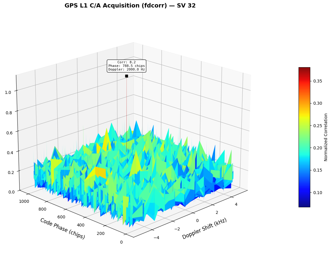
NOTE: Doppler resolution is limited to 1000 Hz in this method (versus previous) and the FFT’ed signal is conjugated (versus the PRN code in previous) which leads to opposite, time-reversed Code Phase output (e.x. code length of $1023 - 788.5 = 234$ ).

fdcorr_loss = 10.0 * np.log10(peak_mag / peak_mag_fdcorr)
print(f"Processing loss of fdcorr() vs traditional approach due to larger doppler bin: {fdcorr_loss:.2f} dB")

Processing loss of fdcorr() vs traditional approach due to larger doppler bin: 0.62 dB

Further improvements can be made to the circular correlation approach below:

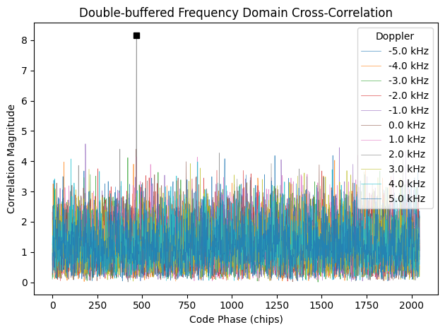
Reuse double-buffered approach from optimal SW FIR filtering to not have to actually circularly shift FFT samples, or create Hankel matrix, but just index/offset the already-FFT’ed samples directly!
Parallelize each correlation (multi-threading with crates like rayon given completely parallel)

sv_idx = 31
sv_fft = prn_fft_sv[sv_idx] # conj(FFT(PRN[sv]))
assert len(sv_fft) == num_corr

sig_fft = np.fft.fft(iq_in[:num_corr])
assert len(sig_fft) == num_corr

# Similar write FFT(signal) to both halfs of a 2x larger buffer
sig_fft_dbl = np.concatenate((sig_fft, sig_fft))
assert len(sig_fft_dbl) == 2 * num_corr

# Limit Doppler search to +/- 5kHz
max_doppler_hz = 5000

doppler_bin_size = fs / num_corr
print(f"Doppler bin size = {doppler_bin_size:.2f} Hz")

# Get whole indices used for frequency shift (NOTE: floor() + 1 useful for symmetrical indices)
num_sym_bins = np.floor(max_doppler_hz / doppler_bin_size)
freq_idx = np.arange(-num_sym_bins, num_sym_bins + 1, dtype=int)
print(f"Frequency indices (shift in Freq domain): {freq_idx}")

# Instead of going through forming whole Hankel matrix, reassigning values, etc.
max_corr = 0.0
freq_offset = 0.0
code_offset = 0
for freq in freq_idx:
    if freq >= 0:
        x_corr_f = sig_fft_dbl[freq:num_corr + freq] * sv_fft
    else: # negative index value, use second half
        x_corr_f = sig_fft_dbl[freq + num_corr:freq + (2*num_corr)] * sv_fft
    x_corr_t = np.abs(np.fft.ifft(x_corr_f))

    freq_bin = freq*doppler_bin_size/1e3
    plt.plot(x_corr_t, linewidth=0.5, alpha=0.8, label=f'{freq_bin} kHz')

    highest_corr = np.max(x_corr_t)
    if highest_corr > max_corr:
        max_corr = highest_corr
        freq_offset = freq_bin
        code_offset = np.argmax(x_corr_t)

print(f"Max corr = {max_corr:.2f} [{freq_offset:.2f} kHz offset | {int(code_offset/2)} code phase]")
plt.plot(code_offset, max_corr, "s", color='black')
plt.legend(loc='upper right', title="Doppler")
plt.title("Double-buffered Frequency Domain Cross-Correlation")
plt.xlabel("Code Phase (chips)")
plt.ylabel("Correlation Magnitude")
plt.tight_layout()
plt.show()

Doppler bin size = 1000.00 Hz Frequency indices (shift in Freq domain): [-5 -4 -3 -2 -1 0 1 2 3 4 5] Max corr = 8.17 [2.00 kHz offset | 234 code phase]

png

Acquisition via Partial Matched Filter + FFT (PMF-FFT)

The PCPS method above searches Doppler in a for loop: every Doppler hypothesis costs one carrier wipe-off plus a forward/inverse FFT pair. The Partial Matched Filter + FFT (PMF-FFT) algorithm is the dual of PCPS — it recovers all Doppler bins at once with a single FFT, exactly the way PCPS recovers all code phases at once with a single FFT. Because it maps cleanly onto a hardware matched filter followed by a small FFT, it is a workhorse acquisition engine in real GPS/GNSS receivers.

Coherent correlation only works once the carrier is removed. With an unknown Doppler $f_{d}$ , the residual carrier rotates during the $T_{coh} = 1\,\text{ms}$ integration, so the correlation collapses along the familiar sinc envelope (the same DFT-bin response described in the PCPS coherent-integration discussion above):

|R(f_{d})| = \big| \text{sinc}(f_{d} \, T_{coh}) \big|, \qquad \text{sinc}(x) = \frac{\sin \pi x}{\pi x}.

At the SV 32 Doppler of

\approx +1.67\,\text{kHz}

the carrier turns

f_{d} T_{coh} \approx 1.67

full cycles over one PRN period, costing $$20\log_{10}

\text{sinc}(1.67)

\approx -16\,\text{dB}$$ — the peak vanishes into the noise. This is precisely why PCPS must wipe the carrier before every single correlation.

The partial-matched-filter trick

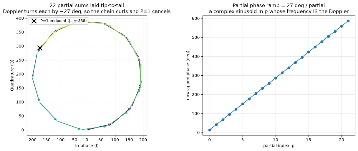
Split the length- $N$ matched filter into $P$ partial correlations (“partial matched filters”), each spanning only $M = N/P$ samples. Suppose the local code is aligned to the true code phase, so after despreading the received samples are a pure tone $z[n] = A\,e^{j(2\pi f_{d} n T_{s} + \phi_{0})}$ (plus noise), with sample period $T_{s} = 1/f_{s}$ . The $p$ -th partial sum is a short geometric series:

y_{p} = \sum_{m=0}^{M-1} z[pM + m] = \underbrace{A\,M\,e^{j\phi_{0}}\, e^{\,j\pi f_{d}(M-1)T_{s}}\,\text{sinc}(f_{d} M T_{s})}_{\text{constant magnitude, same for every } p} \;\cdot\; e^{\,j\,2\pi (f_{d} M T_{s})\, p}.

Two things make this powerful:

Each partial survives the Doppler. A partial spans only $M T_{s} = T_{coh}/P$ seconds, so its own sinc loss $\text{sinc}(f_{d} M T_{s})$ is tiny — for $P = 22$ at $1.67$ kHz it is just $-0.08\,\text{dB}$ .
The Doppler becomes a tone. The partial outputs $y_{0}, y_{1}, \dots, y_{P-1}$ form a discrete complex sinusoid in $p$ whose digital frequency $f_{d} M T_{s}$ depends only on the Doppler. We have converted “find the frequency offset” into “find the frequency of a tone.”

Reading the Doppler with an FFT

A tone is exactly what a DFT detects, so take a $P$ -point FFT across the partials:

Y[k] = \sum_{p=0}^{P-1} y_{p}\, e^{-j 2\pi k p / P}.

All of the partial energy lands in the one bin $k^{\star}$ that matches the rotation rate, and that bin maps directly to Doppler:

f_{d} = \frac{k}{P M T_{s}} = \frac{k}{N T_{s}} = k \cdot \frac{f_{s}}{N}, \qquad k = -\tfrac{P}{2}, \dots, \tfrac{P}{2}-1.

One FFT replaces the entire Doppler loop. Its behaviour follows straight from the DFT:

Property	Expression	GPS L1 C/A ( $N = 2046$ , $P = 22$ )
Doppler bin spacing (resolution)	$\Delta f = 1/T_{coh} = f_{s}/N$	$1000$ Hz
Unambiguous Doppler span	$\pm \dfrac{1}{2 M T_{s}} = \pm \dfrac{P}{2\,T_{coh}}$	$\pm 11$ kHz
Worst-case scalloping (band edge)	$\text{sinc}(1/2) = 2/\pi$	$-3.92$ dB
Scalloping at $\pm 5$ kHz	$\text{sinc}(5000 \cdot M T_{s})$	$-0.75$ dB

The resolution equals PCPS’s coherent limit ( $1/T_{coh}$ ), but the Doppler span grows with the number of partials $P$ : more, shorter partials widen the search and flatten the scalloping envelope, at the cost of a larger FFT.

# === PMF-FFT mechanism (idealized, noise-free) ===
# Show WHY partitioning + FFT recovers a Doppler that destroys a single
# full-length coherent correlation. We use a clean synthetic tone at the
# measured SV 32 Doppler so the geometry is visible; real data follows below.

pmf_P = 22                      # number of partial correlations (must divide N)
N     = num_corr                # 2046 samples = 1 PRN period
pmf_M = N // pmf_P              # 93 samples per partial
T_s   = 1.0 / fs
f_d   = doppler_shifts[peak_dop_idx]   # SV 32 Doppler (Hz) from the PCPS search above

# Despread + perfectly aligned -> a pure Doppler tone (noise-free, for clarity)
n = np.arange(N)
z = np.exp(1j * 2 * np.pi * f_d * n * T_s)

# The P partial sums (each an M-sample "partial matched filter")
y_p = np.array([z[p*pmf_M:(p+1)*pmf_M].sum() for p in range(pmf_P)])

# Full coherent sum == one partial of length N (the P = 1 case): Doppler rotates
# the running sum through > 1.5 turns, so it nearly cancels itself.
coh_P1  = np.abs(z.sum())
sum_mag = np.sum(np.abs(y_p))   # what the partials would give if added in phase
print(f"Single coherent correlation (P=1): |sum| = {coh_P1:7.1f}")
print(f"Sum of partial magnitudes        : {sum_mag:7.1f}"
      f"  ->  P=1 loss = {20*np.log10(coh_P1/sum_mag):+.1f} dB")
print(f"Per-partial dwell = {pmf_M*T_s*1e6:.1f} us, sinc loss = "
      f"{20*np.log10(abs(np.sinc(f_d*pmf_M*T_s))):+.2f} dB (np.sinc is the normalized sinc)")

fig, (axL, axR) = plt.subplots(1, 2, figsize=(13, 5.6))
fig.subplots_adjust(top=0.84, bottom=0.11, left=0.07, right=0.97, wspace=0.26)

# --- Left: the P partials laid tip-to-tail (= the coherent integration path) ---
colors = plt.cm.viridis(np.linspace(0, 1, pmf_P))
verts = np.concatenate([[0], np.cumsum(y_p)])   # chain vertices: 0 -> ... -> full sum
axL.plot(verts.real, verts.imag, "-", color="lightgray", lw=1, zorder=1)  # running sum path
for p in range(pmf_P):
    axL.annotate("", xy=(verts[p+1].real, verts[p+1].imag),
                 xytext=(verts[p].real, verts[p].imag),
                 arrowprops=dict(arrowstyle="->", color=colors[p], lw=1.6), zorder=2)
axL.plot(verts[-1].real, verts[-1].imag, "kx", ms=11, mew=2.5, zorder=3,
         label=f"P=1 endpoint (|.| = {coh_P1:.0f})")
deg_per = 360 * f_d * pmf_M * T_s
axL.set_title(f"{pmf_P} partial sums laid tip-to-tail\n"
              f"Doppler turns each by ~{deg_per:.0f} deg, so the chain curls and P=1 cancels")
axL.set_xlabel("In-phase (I)"); axL.set_ylabel("Quadrature (Q)")
axL.set_aspect("equal"); axL.grid(alpha=0.3); axL.legend(loc="upper left", fontsize=9)

# --- Right: the partial phases form a straight ramp == a tone the FFT finds ---
axR.plot(np.arange(pmf_P), np.degrees(np.unwrap(np.angle(y_p))), "o-", color="C0")
axR.set_title(f"Partial phase ramp = {deg_per:.0f} deg / partial\n"
              f"a complex sinusoid in p whose frequency IS the Doppler")
axR.set_xlabel("partial index  p"); axR.set_ylabel("unwrapped phase (deg)")
axR.grid(alpha=0.3)

plt.show()

Single coherent correlation (P=1): |sum| = 338.4 Sum of partial magnitudes : 2026.7 -> P=1 loss = -15.5 dB Per-partial dwell = 45.5 us, sinc loss = -0.08 dB (np.sinc is the normalized sinc)

png

Computing every code phase efficiently

The mechanism above assumed we already knew the code phase. To search all $N$ code phases simultaneously, compute each partial correlation with an FFT — but window the signal into the $P$ contiguous blocks and correlate each block against the full periodic code:

y_{p}[\phi] = \text{IFFT}\Big\{\, \text{FFT}\{r_{p}\} \cdot \text{FFT}\{c\}^{*} \,\Big\}, \qquad r_{p}[n] = \begin{cases} r[n], & pM \le n < (p{+}1)M \\ 0, & \text{otherwise.} \end{cases}

Windowing the signal rather than the code is the key detail: the PRN code is periodic, so the circular wrap implied by the FFT correlation is exact, while each signal block stays contiguous in time and therefore keeps the clean Doppler phase ramp derived above. The result is the partial-correlation bank $y_{p}[\phi]$ with shape $P \times N$ . Running a length- $P$ FFT down the partial axis for every code phase then produces the full (code phase $\times$ Doppler) acquisition surface. That FFT is usually zero-padded to interpolate a smooth Doppler axis — interpolation only sharpens the peak read-out; the true resolution stays $1/T_{coh}$ .

Compare the cost to PCPS, which pays a full FFT pair for every Doppler bin:

	PCPS (`for` loop over Doppler)	PMF-FFT
Carrier wipe-offs	one per Doppler bin	none
Length- $N$ FFTs / IFFTs	$2 \times N_{\text{Doppler}}$	$\approx 2P$ (signal blocks)
Doppler search	serial, arbitrary bin spacing	one length- $P$ FFT per code phase, fixed $\Delta f = f_{s}/N$
Recovers all Dopplers at once?	no	yes

For the $\pm 5$ kHz / 100-bin search used earlier, PCPS computes $\approx 200$ length- $N$ transforms; the $P = 22$ PMF-FFT computes $\approx 45$ , while also covering the wider $\pm 11$ kHz span. (In dedicated hardware the partials come from a sliding/serial matched-filter correlator, so the code-phase dimension needs no FFTs at all — only the small Doppler FFT remains.)

# === PMF-FFT acquisition on the recorded signal (full 2D surface) ===
pmf_sv     = 32
pmf_prn_up = np.repeat(generate_ca_code(pmf_sv), sps).astype(complex)  # +/-1 code, length N
pmf_n_fft  = 1024                                                      # zero-pad Doppler axis

def pmf_fft_acquire(r, code_up, P, n_fft):
    """Partial-Matched-Filter + FFT acquisition over all code phases and Dopplers.

    Mirrors the derivation above:
      1. window the SIGNAL into P contiguous M-sample blocks,
      2. correlate each block against the full (periodic) code via FFT
         -> partial-correlation bank y_p[phi] of shape (P, N),
      3. FFT (zero-padded) down the partial axis -> Doppler at every code phase.

    Returns |surface| of shape (N code phases, n_fft Doppler bins) and the
    Doppler axis in Hz.
    """
    N = len(code_up)
    M = N // P
    code_fft_conj = np.conj(np.fft.fft(code_up))        # full code spectrum (computed once)
    y_p = np.empty((P, N), dtype=complex)               # partial-correlation bank
    for p in range(P):
        r_block = np.zeros(N, dtype=complex)
        r_block[p*M:(p+1)*M] = r[p*M:(p+1)*M]           # keep block p, zero the rest
        y_p[p] = np.fft.ifft(np.fft.fft(r_block) * code_fft_conj)
    # Doppler search: one FFT down the partial axis covers every code phase at once
    dop = np.fft.fftshift(np.fft.fft(y_p, n=n_fft, axis=0), axes=0)   # (n_fft, N)
    dop_axis = np.fft.fftshift(np.fft.fftfreq(n_fft, d=M / fs))       # Hz
    return np.abs(dop.T), dop_axis                      # (N, n_fft), Hz

pmf_surface, pmf_dop_hz = pmf_fft_acquire(iq_in[:num_corr], pmf_prn_up, pmf_P, pmf_n_fft)

# --- Sanity check: one column must equal the textbook direct partial-sum DFT ---
phi_chk = 468
code_at_phi = np.roll(pmf_prn_up, phi_chk)              # c[(n - phi) mod N]
y_direct = np.array([(iq_in[p*pmf_M:(p+1)*pmf_M] * code_at_phi[p*pmf_M:(p+1)*pmf_M]).sum()
                     for p in range(pmf_P)])
dop_direct = np.fft.fftshift(np.abs(np.fft.fft(y_direct, n=pmf_n_fft)))
assert np.allclose(dop_direct, pmf_surface[phi_chk], atol=1e-9)
print("FFT-accelerated surface matches the direct partial-sum DFT: OK")

# --- Peak of the 2D surface ---
pk = np.unravel_index(np.argmax(pmf_surface), pmf_surface.shape)
pmf_peak_chips   = pk[0] / sps
pmf_peak_doppler = pmf_dop_hz[pk[1]]
pmf_peak_mag     = pmf_surface[pk]
print(f"PMF-FFT peak: corr {pmf_peak_mag:.2f} | "
      f"{pmf_peak_doppler:+.1f} Hz Doppler | {pmf_peak_chips:.1f} chips")

# A single coherent correlation with no carrier wipe-off (the P=1 case),
# evaluated at the SAME acquired code phase -> shows what the Doppler destroyed.
coh_P1 = np.abs(np.fft.ifft(np.fft.fft(iq_in[:num_corr]) * np.conj(np.fft.fft(pmf_prn_up))))
coh_P1_at_peak = coh_P1[pk[0]]
print(f"P=1 (no wipe-off) at this code phase: {coh_P1_at_peak:.2f}  ->  "
      f"partitioning into P={pmf_P} recovers {20*np.log10(pmf_peak_mag/coh_P1_at_peak):+.1f} dB")

# --- Surface plot (same style as the PCPS / fdcorr acquisition surfaces) ---
keep = np.abs(pmf_dop_hz) <= 6000                       # crop to +/-6 kHz for clarity
Zsurf = pmf_surface[:, keep]
Zsurf = Zsurf / Zsurf.max()
X, Y = np.meshgrid(pmf_dop_hz[keep] / 1000, np.arange(num_corr) / sps)

fig = plt.figure(figsize=(14, 9))
ax = fig.add_subplot(111, projection='3d')
surf = ax.plot_surface(X, Y, Zsurf, cmap='jet', rstride=4, cstride=1,
                       antialiased=True, linewidth=0, alpha=0.95)
ax.set_xlabel('Doppler Shift (kHz)', fontsize=12, labelpad=10)
ax.set_ylabel('Code Phase (chips)', fontsize=12, labelpad=10)
ax.set_zlabel('Normalized Correlation', fontsize=12, labelpad=10)
ax.set_title(f'GPS L1 C/A Acquisition (PMF-FFT, P={pmf_P}) - SV {pmf_sv}',
             fontsize=14, fontweight='bold')
ax.view_init(elev=20, azim=225)
ax.set_zlim(0, 1.15)

annotation = (f"Corr: {pmf_peak_mag:.1f}\n"
              f"Phase: {pmf_peak_chips:.1f} chips\n"
              f"Doppler: {pmf_peak_doppler:.1f} Hz")
ax.text(pmf_peak_doppler / 1000, pmf_peak_chips, 1.05, annotation,
        fontsize=8, fontfamily='monospace', ha='center', va='bottom',
        bbox=dict(boxstyle='round,pad=0.4', facecolor='white', edgecolor='black', alpha=0.85),
        zorder=10)

fig.colorbar(surf, shrink=0.55, aspect=12, pad=0.1, label='Normalized Correlation')
plt.tight_layout()
plt.show()

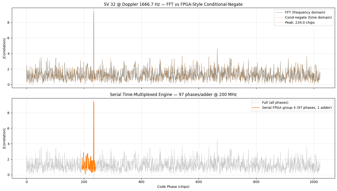
FFT-accelerated surface matches the direct partial-sum DFT: OK PMF-FFT peak: corr 9.43 | +1675.8 Hz Doppler | 234.0 chips P=1 (no wipe-off) at this code phase: 1.80 -> partitioning into P=22 recovers +14.4 dB

png

Pros, cons, and design choices

Advantages over PCPS:

No per-Doppler carrier wipe-off and no Doppler for loop. The whole Doppler dimension comes from one small FFT, so the expensive length- $N$ transforms are paid once per signal block instead of twice per Doppler bin.
Hardware friendly. The partial correlations are exactly what a sliding/serial matched-filter ASIC or FPGA already produces; bolting a short FFT (or even a handful of DFT twiddle multiplies) onto its output yields the full Doppler search almost for free. This is the classic GNSS acquisition architecture.
Wide Doppler span at little extra cost. Adding partials widens the unambiguous span ( $\pm P/2\,T_{coh}$ ) without any extra correlation work — handy for cold starts or high-dynamics users where the Doppler uncertainty is large.

Disadvantages / costs:

Scalloping (straddle) loss. The per-partial $\text{sinc}(f_{d} M T_{s})$ envelope rolls off toward the band edge — up to $-3.9$ dB worst case. Mitigate by using more (shorter) partials so the Doppler range of interest sits inside the flat part of the main lobe, and by zero-padding the FFT to reduce the bin-straddle component.
Fixed Doppler resolution. Bin spacing is locked to $1/T_{coh}$ by the coherent integration time, whereas PCPS can pick an arbitrarily fine Doppler grid. Zero-padding only interpolates; it does not narrow the true main lobe.
Code phase still needs a search. PMF-FFT elegantly parallelizes Doppler; the code-phase dimension is still handled by the (FFT-based or sliding) partial correlators, just as in PCPS.
Boundary sensitivity. $P$ must divide $N$ (or the code/data is zero-padded so it does), and a navigation-data-bit edge landing inside the coherent window still corrupts the partials — capping $T_{coh}$ at one data symbol (20 ms for GPS) unless bit-edge handling or non-coherent integration is added.

Choosing $P$ : pick the smallest $P$ whose span $\pm P/2\,T_{coh}$ comfortably covers your Doppler uncertainty while keeping the edge scalloping acceptable. Larger $P$ widens the span and flattens scalloping, but enlarges both the FFT and the partial-correlator bank. For this $\pm 5$ kHz GPS search, $P = 22$ (span $\pm 11$ kHz, edge-of-interest loss $-0.75$ dB) is a good balance. Note above that the PMF-FFT peak ( $\approx 9.4$ ) recovers essentially the same processing gain as the PCPS surface — it just reaches it with one Doppler FFT instead of a hundred carrier wipe-offs, and the DSSS processing gain of $10\log_{10}(N)$ is preserved because the FFT recombines the partials coherently.

FPGA Dataflow: A Streaming PMF-FFT Acquisition Engine

The “hardware friendly” claim deserves substantiation. Below is the complete dataflow of a streaming PMF-FFT engine as built in real GNSS ASICs/FPGAs, sized with concrete numbers for GPS L1 C/A: $N = 2046$ samples per PRN period, $P = 22$ partials of $M = N/P = 93$ samples, FFT length $K = 32$ (the next power of two $\geq P$ — recall from the runtime comparison below that any larger $K$ only interpolates), input rate $f_s = 2.046$ Msps, fabric clock $f_{clk} = 200$ MHz.

In plain words, the machine does this: for every possible code alignment, multiply 1 ms of input samples by a local $\pm 1$ code copy and add them up — but instead of one big sum per alignment, keep $P = 22$ consecutive sub-sums (the “partials”). If the alignment is right, the partials trace out a slow spiral whose rotation rate is the Doppler; a tiny FFT across the 22 partials reads that rate out directly. No mixer, no carrier NCO, no Doppler loop — the FFT stage replaces all of them. Crucially, hardware computes the partials directly in the time domain (the y_direct sanity-check in the acquisition cell above is this datapath, making it a bit-true golden model), so none of the per-block length- $N$ FFTs from the software version exist here.

This architecture is the performance/resource optimum for three reasons:

The correlation — over 99% of the arithmetic — costs zero DSP slices. Chips are $\pm 1$ , so “multiply by code” degenerates to a 2:1 MUX + conditional negate (dissected in its own section below), and the partial sums are plain fabric adders.
The only multipliers live in a tiny, massively under-utilized FFT. One serial radix-2 butterfly (1 complex multiplier $\approx$ 3 DSP slices) needs $\approx 7{,}400$ cycles per 1 ms PRN period against $200{,}000$ available — 25 $\times$ headroom. The entire Doppler dimension costs about 5 DSP slices.
Time-multiplexing is the resource $\leftrightarrow$ speed dial. With $\lfloor f_{clk}/f_s \rfloor = 97$ clock cycles available per input sample, one physical accumulator lane can service $C$ code-phase hypotheses per pass; we choose $C = 93$ so that $N/C = 22$ passes exactly cover all code phases (and the buffer depth becomes a clean 2046 words). A full single-SV cold-start search takes $22 \times T_{PRN} = 22$ ms; replicating the fabric-cheap correlator bank $R\times$ cuts that to $22/R$ ms or searches $R$ SVs in parallel. (That $C = 93$ equals $M = 93$ is numeric coincidence — they are unrelated parameters.)

                            x[n]: 4b I + 4b Q complex samples @ f_s = 2.046 Msps
                            │  (async input FIFO = the only clock-domain crossing;
                            │   everything below runs on one f_clk = 200 MHz)
                            ▼
   ┌─────────────────────────────────────────────────┐
   │ ADC SAMPLE REGISTER                             │
   │ holds x[n] steady for C = 93 f_clk cycles       │
   └────────────────────────┬────────────────────────┘
                            │ x[n]
                            ▼
   ┌─────────────────────────────────────────────────┐
   │ CODE "MULTIPLY": 2:1 MUX + conditional negate   │
   │   code bit = 0  →  +x[n]                        │◄── code bit c[(n−φᵢ) mod N] from an N × 1b
   │   code bit = 1  →  −x[n]                        │    code ROM, filled at boot by the G1/G2
   │ (0 DSP slices — pure LUT logic)                 │    LFSRs (any SV 1-37). The ROM address
   └────────────────────────┬────────────────────────┘
                                                          needs no math: it decrements once per
                                                          f_clk cycle and reloads at +1 per
                                                          sample — just two mod-N counters.
                            │ ±x[n]  (5b I + 5b Q)
                            ▼
   ┌─────────────────────────────────────────────────┐
   │ ACCUMULATOR BANK: C = 93 complex accumulators   │
   │ (LUTRAM/FF, 11b I + 11b Q each — 0 DSP)         │
   │ f_clk cycle i of each sample, i = 0..C−1:       │
   │   acc[i] += ±x[n]   (code phase φᵢ = pass·C+i)  │
   └────────────────────────┬────────────────────────┘
                            │ every M = 93 samples (block boundary, partial
                            │ index p = ⌊n/M⌋ = 0..P−1): dump all C partial
                            │ sums y_p[φᵢ] as one row, clear accumulators
                            ▼
   ┌─────────────────────────────────────────────────┐
   │ PARTIAL-SUM BUFFER (ping-pong)                  │
   │ 2 × [ P·C = 22 × 93 = 2046 words × 22b ] BRAM   │
   │ row p ← the C partials dumped at boundary p     │
   └────────────────────────┬────────────────────────┘
                            │ side A fills over one PRN period (1 ms) while
                            │ the FFT drains side B: per phase φᵢ, read its
                            │ P = 22 partials down a column, then feed
                            │ K − P = 10 zeros (zero-padding)
                            ▼
   ┌─────────────────────────────────────────────────┐
   │ K = 32-POINT FFT                                │
   │ radix-2, ONE serial butterfly, in-place:        │◄── twiddle ROM, K/2 × (16b+16b) (LUT ROM)
   │ 1 complex multiplier  =  3 DSP slices           │
   │ load: 93 FFTs/ms ≈ 7.4k of 200k f_clk cycles    │
   └────────────────────────┬────────────────────────┘
                            │ Y[k]: K = 32 Doppler bins per phase, 16b+16b
                            ▼
   ┌─────────────────────────────────────────────────┐
   │ MAGNITUDE + INTEGRATION                         │
   │ |Y[k]|² = I·I + Q·Q          (2 DSP slices)     │
   │ optional: non-coherent sum over L PRN periods   │
   │ for weak signals (C·K × 32b BRAM)               │
   └────────────────────────┬────────────────────────┘
                            ▼
   ┌─────────────────────────────────────────────────┐
   │ PEAK + THRESHOLD SEARCH                         │
   │ running max & argmax → (φ_pk, k_pk)             │
   │ running sum Σ over all searched cells           │
   │ declare detection when  max > T · Σ/(C·K)       │
   └────────────────────────┬────────────────────────┘
                            │
                            ├─► code phase  =  φ_pk samples          → seeds DLL
                            └─► Doppler f_d =  k_pk · f_s/N  Hz      → seeds PLL
                                (read k_pk as a SIGNED 5-bit int: bins k ≥ K/2
                                 are negative Dopplers — a free "fftshift")

Control is four counters in one synchronous process — there are no handshakes and no backpressure anywhere; every block advances on counter state with fixed latency:

 i     0..C−1     f_clk cycle within the current sample  →  which acc[i] is serviced
 n     0..N−1     sample index within the PRN period     →  code ROM base address
 p     0..P−1     p = ⌊n/M⌋; (n mod M == M−1) marks a block boundary → dump row p, clear accs
 pass  0..N/C−1   which group of C code phases is in flight (φᵢ = pass·C + i);
                  increments every PRN period → 22 passes = full code-phase search

The ping-pong partial buffer is what decouples the sample-rate correlator from the burst-rate FFT engine:

correlator:  |◄─── PRN period q: fills side A ───────────────►|◄─── period q+1: fills side B ───
             | block 0 | block 1 |  ...  | block 20 | block 21|
             |         ↑ dump row 0                 ↑ row 20  ↑ row 21 → side A full, swap sides
FFT engine:  |◄─── drains side B (period q−1 partials) ──────►|◄─── drains side A ──────────────
             |     93 phases × one 32-pt FFT each ≈ 7.4k of the 200k f_clk cycles available

Bit-width plan (all signed two’s complement; these are the numbers the HDL actually needs):

Node	Width (I + Q)	Sizing rule
input `x[n]`	4 + 4	2-4 bits is standard for GNSS; front-end AGC keeps RMS noise near ~2 LSBs
`±x[n]`	5 + 5	negating −8 requires one extra bit
partial `y_p`	11 + 11	max magnitude is $93 \times 8 = 744 < 2^{10}$ , i.e. $\lceil \log_2 (M \cdot 2^4) \rceil + 1$ sign bit
FFT output `Y[k]`	16 + 16	coherent bit growth $\leq \lceil \log_2 P \rceil = 5$ (only $P$ of the $K$ inputs are nonzero)
`abs(Y)²`	32	$16 \times 16 \rightarrow 31$ b products, plus one bit for the I²+Q² add
non-coherent sum	32 + $\lceil \log_2 L \rceil$	grows with the number of PRN periods $L$ summed

Resource budget (one engine, $R = 1$ , 7-series/UltraScale-class estimates):

Block	LUT / FF	BRAM36	DSP
G1/G2 code LFSRs + N × 1b code ROM	~50 FF	1	0
MUX-negate + adder + C-deep accumulator bank	~1-2k LUT	0	0
partial ping-pong buffer (2 × 2046 × 22b)	—	4	0
32-pt serial FFT (butterfly + twiddle ROM + control)	~500 LUT	0	3
`abs(Y)²` magnitude	—	0	2
non-coherent surface (optional, 93 × 32 × 32b)	—	3	0
peak / threshold search	~100 LUT	0	0
Total	a few k LUT	~5-8	5

For contrast, a PCPS engine at the same update rate needs a full streaming length- $N$ FFT/IFFT core (tens of DSP slices and BRAMs) plus a complex NCO and mixer, exercised once per Doppler bin — the engine above replaces all of that with five DSP slices, and its Doppler span ( $\pm 11$ kHz) is set by $P$ , not by how many times you can afford to rerun a big FFT.

HDL implementation checklist:

One clock domain. The input async FIFO is the only clock-domain crossing; downstream, the four counters schedule everything deterministically — no ready/valid plumbing.
Dump-and-clear is free: at a block boundary the accumulator write mux selects load (acc[i] <= ±x) instead of accumulate (acc[i] <= acc[i] ± x) — clearing costs no extra cycle.
Code ROM contents: the $\pm 1$ code pre-upsampled to the sample rate (each chip repeated sps = 2 times), one bit per entry (0 → +1, 1 → −1). Boot-time fill from the ~20-flip-flop G1/G2 LFSR generator lets one engine acquire any SV.
FFT options: vendor streaming FFT IP configured for $K = 32$ works, but at this size a hand-rolled in-place radix-2 (single butterfly, 5 stages, 16-entry twiddle ROM) — or even a direct $P$ -input DFT — is equally fine. Zero-padding is literally “feed 10 zeros after the 22 partials.”
Doppler sign for free: interpret the peak bin index as a signed 5-bit integer — upper bins are negative Dopplers. This replaces the software fftshift with a type cast.
Detection: compare the peak against $T \times$ the mean of all searched cells with $T \approx 2$ -3 (the same peak-to-floor metric used in the correlator sections below), or against a calibrated noise floor; enable the non-coherent accumulator when hunting weak signals.
Verification: quantize this notebook’s iq_in to your chosen input width and pmf_fft_acquire() — or the direct y_direct partial-sum check, which mirrors the hardware dataflow exactly — becomes a bit-true golden reference: dump y_p and Y[k] from RTL simulation and diff.

PMF-FFT References

D. J. R. van Nee and A. J. R. M. Coenen, “New fast GPS code-acquisition technique using FFT,” Electronics Letters, vol. 27, no. 2, pp. 158-160, 1991 — the origin of FFT-based GPS acquisition.
K. Borre, D. M. Akos, N. Bertelsen, P. Rinder, and S. H. Jensen, A Software-Defined GPS and Galileo Receiver: A Single-Frequency Approach, Birkhauser, 2007 — derives the parallel code-phase and parallel-frequency (FFT) acquisition methods with MATLAB.
J. B.-Y. Tsui, Fundamentals of Global Positioning System Receivers: A Software Approach, 2nd ed., Wiley, 2005 — Chapters on acquisition cover the averaging/partial-correlation + FFT approach in detail.
GNSS-SDR acquisition documentation — production implementations of PCPS and PMF/FFT-style acquisition blocks.

Runtime Comparison of Frequency-Domain Methods

All three methods above land on the same answer for SV 32 (code phase $\approx 234$ chips, Doppler $\approx +1.7$ kHz), so the remaining question is what each costs. The cell below times realistic implementations of just the core search (single SV, one PRN period of $N = 2046$ samples, $\pm 5$ kHz Doppler), excluding everything a real receiver precomputes once and reuses across acquisition attempts:

The conjugated, FFT’d PN spreading code $\text{conj}(\text{FFT}(\text{PRN}))$ — computed once per SV and stored (as in the prn_fft_sv table built earlier).
The PCPS carrier wipe-off phasor bank — the Doppler search grid is fixed, so the complex exponentials are shared by every SV and every acquisition attempt.

PMF-FFT is timed two ways: with the heavily zero-padded $n_{fft} = 1024$ Doppler FFT used for the smooth surface plot above, and with a realistic $n_{fft} = 32$ — the FFT only needs $\geq P = 22$ points to resolve every Doppler bin the partial sums can actually distinguish; the extra zero-padded points are pure spectral interpolation for plotting.

# === Acquisition runtime comparison: PCPS vs double-buffered vs PMF-FFT ===
import timeit

bench_sv_fft = prn_fft_sv[31]     # conj(FFT(PRN)) for SV 32 — precomputed once per SV
bench_r      = iq_in[:num_corr]   # one PRN period (1 ms) of received I/Q
bench_N      = num_corr

# PCPS: the Doppler search grid is fixed, so a real receiver also precomputes the
# carrier wipe-off phasor bank (reused for every SV and every acquisition attempt)
bench_t       = np.arange(bench_N) / fs
wipeoff_bank  = np.exp(-1j * 2 * np.pi * doppler_shifts[:, None] * bench_t[None, :])

def acquire_pcps():
    """Traditional PCPS: per Doppler bin, wipe off carrier in time domain then FFT correlate."""
    best_mag, best_dop, best_phase = 0.0, 0.0, 0
    for d in range(len(doppler_shifts)):
        corr = np.abs(np.fft.ifft(np.fft.fft(bench_r * wipeoff_bank[d]) * bench_sv_fft))
        idx = int(np.argmax(corr))
        if corr[idx] > best_mag:
            best_mag, best_dop, best_phase = corr[idx], doppler_shifts[d], idx
    return best_mag, best_dop, best_phase

db_bin_hz   = fs / bench_N                  # 1 kHz Doppler per FFT-index shift
db_freq_idx = np.arange(-5, 6, dtype=int)   # +/-5 kHz -> 11 bins

def acquire_dbl_buf():
    """Double-buffered joint search: one signal FFT, Doppler = circular slice of the double buffer."""
    sig_fft = np.fft.fft(bench_r)
    sig_dbl = np.concatenate((sig_fft, sig_fft))
    best_mag, best_dop, best_phase = 0.0, 0.0, 0
    for f in db_freq_idx:
        sl = sig_dbl[f:bench_N + f] if f >= 0 else sig_dbl[f + bench_N:f + 2 * bench_N]
        corr = np.abs(np.fft.ifft(sl * bench_sv_fft))
        idx = int(np.argmax(corr))
        if corr[idx] > best_mag:
            best_mag, best_dop, best_phase = corr[idx], f * db_bin_hz, idx
    return best_mag, best_dop, best_phase

def acquire_pmf_fft(n_fft):
    """PMF-FFT: P partial correlations via FFT, then one batched FFT down the partial axis."""
    M = bench_N // pmf_P
    y_p = np.empty((pmf_P, bench_N), dtype=complex)
    r_block = np.zeros(bench_N, dtype=complex)
    for p in range(pmf_P):
        r_block[:] = 0
        r_block[p * M:(p + 1) * M] = bench_r[p * M:(p + 1) * M]
        y_p[p] = np.fft.ifft(np.fft.fft(r_block) * bench_sv_fft)
    surf = np.abs(np.fft.fft(y_p, n=n_fft, axis=0))
    pk = np.unravel_index(np.argmax(surf), surf.shape)
    return surf[pk], np.fft.fftfreq(n_fft, d=M / fs)[pk[0]], pk[1]

candidates = [
    ("PCPS (100 bins)",            acquire_pcps),
    ("Double-buffered (11 bins)",  acquire_dbl_buf),
    ("PMF-FFT (n_fft=1024)",       lambda: acquire_pmf_fft(pmf_n_fft)),
    ("PMF-FFT (n_fft=32)",         lambda: acquire_pmf_fft(32)),
]

results = []
for name, fn in candidates:
    mag, dop_hz, phase = fn()  # warm-up run; also used for the agreement check
    t_ms = np.median(timeit.repeat(fn, number=1, repeat=15)) * 1e3
    results.append((name, t_ms, mag, dop_hz, phase))

# All methods must agree within their bin resolutions: code phase to within one
# chip (coarser Doppler bins shift the sub-sample correlation peak slightly) and
# Doppler to within half the coarsest bin (1 kHz)
ref_phase = results[0][4]
for name, _, _, dop_hz, phase in results:
    assert abs(phase - ref_phase) <= sps, f"{name} code phase {phase} != {ref_phase}"
    assert abs(dop_hz - results[0][3]) <= 500, f"{name} Doppler {dop_hz} disagrees"
print(f"All methods agree: code phase {ref_phase / sps:.1f} chips, "
      f"Doppler ~{results[0][3]:.0f} Hz\n")

t_pcps = results[0][1]
print(f"{'Method':<28} {'Median time':>12} {'vs PCPS':>9}   Peak (Hz @ chips)")
print("-" * 75)
for name, t_ms, mag, dop_hz, phase in results:
    print(f"{name:<28} {t_ms:>9.2f} ms {t_pcps / t_ms:>8.1f}x   "
          f"{dop_hz:+7.1f} @ {phase / sps:6.1f}")

All methods agree: code phase 234.0 chips, Doppler ~1667 Hz Method Median time vs PCPS Peak (Hz @ chips) --------------------------------------------------------------------------- PCPS (100 bins) 8.57 ms 1.0x +1666.7 @ 234.0 Double-buffered (11 bins) 0.60 ms 14.4x +2000.0 @ 234.5 PMF-FFT (n_fft=1024) 19.71 ms 0.4x +1675.8 @ 234.0 PMF-FFT (n_fft=32) 2.19 ms 3.9x +1375.0 @ 234.0

The measured ordering follows directly from counting length- $N$ FFTs, since each is $\mathcal{O}(N \log N)$ and everything else (wipe-off multiplies, spectrum multiplies, magnitude passes) is a linear $\mathcal{O}(N)$ pass:

Method	Core complexity	Length- $N$ FFTs	Why the result is expected
PCPS	$\mathcal{O}(N_d \cdot N \log N)$	$\approx 200$	Every one of the $N_d = 100$ Doppler bins pays its own carrier wipe-off multiply, forward FFT, spectrum multiply, and IFFT. Runtime is linear in the number of Doppler bins — and PCPS searches the finest grid here ( $\approx 101$ Hz bins).
Double-buffered	$\mathcal{O}((1 + N_d) \cdot N \log N)$	$\approx 12$	The signal is FFT’d once; each Doppler hypothesis is just a circularly-shifted slice of the double buffer, leaving only a spectrum multiply + IFFT per bin. The DFT shift property also quantizes bins to $f_s/N = 1$ kHz, so only $N_d = 11$ bins cover $\pm 5$ kHz. Fewer FFTs per bin $\times$ ~ $9\times$ fewer bins compounds to the order-of-magnitude win — paid for with coarse 1 kHz Doppler resolution (the scalloping loss measured earlier).
PMF-FFT ( $n_{fft} = 1024$ )	$\mathcal{O}(P \cdot N \log N + N \cdot K \log K)$	$44$ + Doppler FFTs	The $P = 22$ partial correlations cost 2 transforms each, but the Doppler stage is a $K = 1024$ -point FFT at every one of the $N = 2046$ code phases — a batched $\approx 2$ M-point workload that dwarfs everything else and makes the pretty-plot configuration the slowest of all.
PMF-FFT ( $n_{fft} = 32$ )	$\mathcal{O}(P \cdot N \log N + N \cdot K \log K)$	$44$ + tiny Doppler FFTs	Same partial-correlation cost, but shrinking $K$ from $1024 \rightarrow 32$ makes the Doppler stage negligible; total work $\approx 44$ length- $N$ FFTs, landing between double-buffered and PCPS — while covering the widest Doppler span ( $\pm f_s / 2M = \pm 11$ kHz) with no wipe-off loop at all.

Caveat: these wall-clock times measure NumPy’s vectorized FFT throughput plus Python loop overhead, which tracks the FFT-count analysis well — but software timing understates PMF-FFT’s appeal in hardware. In an FPGA/ASIC the partial sums fall out of a streaming time-domain correlator (no per-block FFTs at all, and multiplier-free for $\pm 1$ codes per the conditional-negate architecture below), with only a tiny $K$ -point FFT appended; PCPS instead needs full $N$ -point transform throughput per Doppler bin.

Time Domain Acquisition via Direct Matched Filter

All the methods above perform correlation in the frequency domain (multiply-accumulate of FFT bins). We can also acquire GPS signals entirely in the time domain using a direct matched filter, which is conceptually the simplest approach: for each Doppler hypothesis, wipe the carrier, then correlate with the PRN code at every possible code phase by sliding the code across the signal sample-by-sample — identical to an FIR matched filter:

y[n] = \sum_{k=0}^{N-1} r[(n+k) \bmod N] \cdot c[k]

where $r[n]$ is the carrier-wiped received signal and $c[k]$ is the upsampled PRN code. This is circular cross-correlation — the same operation the FFT method computes via $\text{IFFT}\{\text{FFT}\{r\} \cdot \text{FFT}\{c\}^{*}\}$ . To implement it as a sliding dot-product (FIR-style), we tile the input signal so the window naturally wraps around without explicit modular indexing:

r_tiled = [r[0], r[1], ..., r[N-1], r[0], r[1], ..., r[N-1]]
y[n]    = dot(r_tiled[n : n+N], c)   for n = 0, 1, ..., N-1

This is $\mathcal{O}(N^2)$ per Doppler bin (versus $\mathcal{O}(N \log N)$ for the FFT method), so it is significantly slower for long codes, but it maps directly to hardware FIR filter implementations and is useful for understanding what the frequency domain methods are actually computing.

# Time-domain matched filter acquisition for SV 32 (index 31)
sv_num = 32
prn_code_td = generate_ca_code(sv_num)
# Upsample PRN code to match input sample rate
prn_up_td = np.repeat(prn_code_td, sps).astype(complex)

# Doppler search range: same as the traditional frequency-domain method
doppler_shifts_td = np.linspace(-5000, 5000, 100)

# Correlation surface: [doppler bins x code phase bins]
corr_surface_td = np.zeros((len(doppler_shifts_td), num_corr))

for dop_idx, doppler_hz in enumerate(doppler_shifts_td):
    # Carrier wipeoff (identical to frequency-domain method)
    t = np.arange(num_corr) / fs
    carrier_wipeoff = np.exp(-1j * 2 * np.pi * doppler_hz * t)
    wiped_signal = iq_in[:num_corr] * carrier_wipeoff

    # Tile the carrier-wiped signal so the sliding window wraps around,
    # giving us circular cross-correlation as an FIR-style operation.
    wiped_tiled = np.tile(wiped_signal, 2)

    # np.correlate computes: y[n] = sum_k conj(prn[k]) * wiped_tiled[n+k]
    # With the tiled input (length 2N) and code (length N), 'valid' mode
    # slides the code across all N circular offsets — this is the matched
    # filter (FIR convolution with time-reversed conjugate code).
    corr_out = np.correlate(wiped_tiled, prn_up_td, mode='valid')[:num_corr]

    corr_surface_td[dop_idx, :] = np.abs(corr_out)

# --- Surface plot (same style as frequency-domain acquisition) ---
Z_td = corr_surface_td / np.max(corr_surface_td)

x_td = np.arange(num_corr) / sps           # Code phase in chips
y_td = doppler_shifts_td / 1000             # Doppler in kHz
X_td, Y_td = np.meshgrid(x_td, y_td)

fig = plt.figure(figsize=(14, 9))
ax = fig.add_subplot(111, projection='3d')

surf = ax.plot_surface(
    X_td, Y_td, Z_td,
    cmap='jet',
    rstride=1,
    cstride=4,
    antialiased=True,
    linewidth=0,
    alpha=0.95,
)

ax.set_xlabel('Code Phase (chips)', fontsize=12, labelpad=10)
ax.set_ylabel('Doppler Shift (kHz)', fontsize=12, labelpad=10)
ax.set_zlabel('Normalized Correlation', fontsize=12, labelpad=10)
ax.set_title(f'GPS L1 C/A Acquisition (Time-Domain Matched Filter) — SV {sv_num}', fontsize=14, fontweight='bold')
ax.view_init(elev=15, azim=225)
ax.set_zlim(0, 1.15)

# Find and annotate peak
peak_dop_idx_td, peak_phase_idx_td = np.unravel_index(np.argmax(corr_surface_td), corr_surface_td.shape)
peak_phase_chips_td = peak_phase_idx_td / sps
peak_doppler_hz_td = doppler_shifts_td[peak_dop_idx_td]
peak_mag_td = corr_surface_td[peak_dop_idx_td, peak_phase_idx_td]

annotation = (
    f"Corr: {peak_mag_td:.1f}\n"
    f"Phase: {peak_phase_chips_td:.1f} chips\n"
    f"Doppler: {peak_doppler_hz_td:.1f} Hz"
)
ax.text(
    peak_phase_chips_td, peak_doppler_hz_td / 1000, 1.12,
    annotation,
    fontsize=8, fontfamily='monospace',
    ha='center', va='bottom',
    bbox=dict(boxstyle='round,pad=0.4', facecolor='white', edgecolor='black', alpha=0.85),
    zorder=10,
)
ax.plot(
    [peak_phase_chips_td, peak_phase_chips_td],
    [peak_doppler_hz_td / 1000, peak_doppler_hz_td / 1000],
    [1.0, 1.12],
    color='black', linewidth=1, linestyle='--', zorder=9,
)

fig.colorbar(surf, shrink=0.55, aspect=12, pad=0.1, label='Normalized Correlation')
plt.tight_layout()
plt.show()

print(f"\nTime-domain peak: Phase={peak_phase_chips_td:.1f} chips, Doppler={peak_doppler_hz_td:.1f} Hz, Corr={peak_mag_td:.1f}")
print(f"Freq-domain peak (traditional): Phase={peak_phase_chips:.1f} chips, Doppler={doppler_shifts[peak_dop_idx]:.1f} Hz, Corr={peak_mag:.1f}")

png

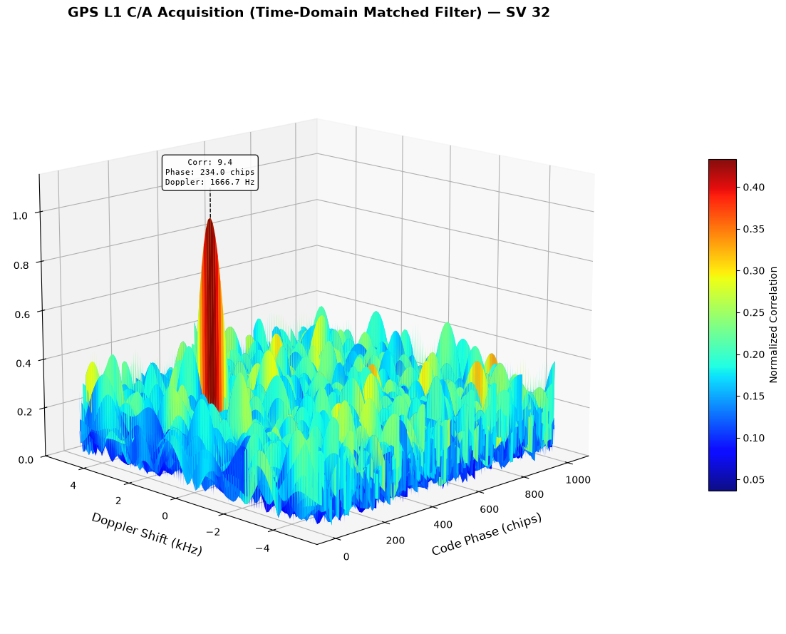
Time-domain peak: Phase=234.0 chips, Doppler=1666.7 Hz, Corr=9.4 Freq-domain peak (traditional): Phase=234.0 chips, Doppler=1666.7 Hz, Corr=9.4

FPGA-Efficient Time-Domain Correlator: Conditional-Negate Architecture

Since GPS C/A code chips $c[k] \in \{+1, -1\}$ , the correlation multiply-accumulate $\text{acc} \mathrel{+}= c[k] \cdot x[k]$ reduces to a conditional negate:

c[k] \cdot x[k] = \begin{cases} +x[k] & \text{if } c[k] = +1 \\ -x[k] & \text{if } c[k] = -1 \end{cases}

On an FPGA this is a 2:1 MUX + adder — zero DSP slice consumption. The entire matched filter runs in fabric (LUTs and registers only):

  ┌──────────────────────── Single Correlator Channel ───────────────────────┐
  │                                                                          │
  │   x[n] ──────────┬──────────┐                                            │
  │   (sample)       │          │                                            │
  │                  │    ┌─────▼─────┐                                      │
  │                  │    │  Negate   │                                      │
  │                  │    │  (-x[n])  │                                      │
  │                  │    └─────┬─────┘                                      │
  │                  │          │                                            │
  │                  ▼          ▼                                            │
  │               ┌────────────────┐         ┌──────────────┐                │
  │    c[k] ─────►│   MUX (1-bit)  │────────►│    Adder     │──► acc[φ]      │
  │   (code ROM)  │  sel: +x / -x  │         │  acc += ±x   │                │
  │               └────────────────┘         └──────┬───────┘                │
  │                                                 │  ▲                     │
  │                                                 └──┘                     │
  │                                              (feedback)                  │
  │                                                                          │
  │   After N samples: dump |acc|² → correlation magnitude, reset acc        │
  └──────────────────────────────────────────────────────────────────────────┘

Time-Multiplexed Serial Architecture

Since the FPGA clock $f_\text{clk}$ is much faster than the input sample rate $f_s$ , we get $M = \lfloor f_\text{clk} / f_s \rfloor$ clock cycles between consecutive input samples. Rather than instantiating $N$ parallel correlators (one per code phase), we time-multiplex $M$ phase hypotheses through a single add/sub unit:

  x[n] held     ┌────────────┐    ┌─────────────┐    ┌─────────────────────┐
  for M clks ──►│ MUX (+/-)  ├───►│   Adder     ├───►│  Accumulator Bank   │
                └─────▲──────┘    └─────────────┘    │  acc[φ₀]            │
                      │                              │  acc[φ₁]            │
                 Code ROM                            │  acc[φ₂]            │
                 (indexed by                         │   ...               │
                  phase φᵢ at                        │  acc[φ_{M-1}]       │
                  each FPGA clk)                     └──────────┬──────────┘
                                                                │
               clk 0 → acc[φ₀] += ±x[n]                         │
               clk 1 → acc[φ₁] += ±x[n]       After N samples:  │
               clk 2 → acc[φ₂] += ±x[n]       M correlations ◄──┘
                ...                             ready
               clk M-1 → acc[φ_{M-1}] += ±x[n]

Each group of $M$ phases completes in one PRN period ( $T_\text{PRN}$ ). To search all $N$ code phase offsets:

T_\text{search} = \left\lceil \frac{N}{M} \right\rceil \cdot T_\text{PRN}

Resource	Parallel (N correlators)	Serial Time-Multiplexed
Adders / Subtractors	$N$	$\lceil N/M \rceil$
Accumulator registers	$N$	$N$
DSP slices	0	0
Code ROM reads/cycle	$N$	1
Search time	$1 \times T_\text{PRN}$	$\lceil N/M \rceil \times T_\text{PRN}$

# === FPGA-Style Conditional-Negate Correlator ===
# Proves that GPS C/A correlation needs zero multiplications:
# only addition, subtraction, and a 1-bit MUX select.

sv_num = 32
prn_code_hw = generate_ca_code(sv_num)
prn_up_hw = np.repeat(prn_code_hw, sps)  # {+1, -1} int8 values

# Carrier wipeoff at the known peak Doppler (from freq-domain result) for verification
peak_doppler_hz_ref = doppler_shifts[peak_dop_idx]
t_ref = np.arange(num_corr) / fs
wiped_signal_ref = iq_in[:num_corr] * np.exp(-1j * 2 * np.pi * peak_doppler_hz_ref * t_ref)

N = num_corr  # 2046 samples per PRN period

# --- Conditional-negate circular correlation (no multiplies) ---
# Precompute masks: which taps add vs subtract
plus_mask = (prn_up_hw == 1)
minus_mask = ~plus_mask

wiped_tiled = np.tile(wiped_signal_ref, 2)
corr_cond_negate = np.zeros(N, dtype=complex)

for phi in range(N):
    window = wiped_tiled[phi:phi + N]
    # The FPGA operation: route each sample to adder (+) or subtractor (-)
    # based on the 1-bit code chip. No multiply anywhere.
    corr_cond_negate[phi] = np.sum(window[plus_mask]) - np.sum(window[minus_mask])

# --- FFT reference for comparison ---
corr_fft_ref = np.fft.ifft(
    np.fft.fft(wiped_signal_ref) * np.conj(np.fft.fft(prn_up_hw.astype(complex)))
)

# Verify exact match (up to floating point)
max_err = np.max(np.abs(corr_cond_negate - corr_fft_ref))
print(f"Max error vs FFT reference: {max_err:.2e} (should be ~machine epsilon × N)")

# --- Serial Time-Multiplexed FPGA Model ---
# One adder services M phase hypotheses per sample period.
f_clk = 200e6  # typical FPGA clock
M = int(f_clk / fs)  # clocks available per input sample
num_groups = int(np.ceil(N / M))

print(f"\nFPGA Architecture @ f_clk = {f_clk/1e6:.0f} MHz, f_s = {fs/1e6:.3f} MHz:")
print(f"  Clocks per sample (M):          {M}")
print(f"  Phases per add/sub unit:         {M}")
print(f"  Add/sub units for all {N} phases: {num_groups}")
print(f"  Full search time:                {num_groups} PRN periods ({num_groups} ms)")
print(f"  DSP slices required:             0")

# Model the serial engine for the group of M phases containing the expected peak
peak_phase_sample = int(peak_phase_chips * sps)
group_id = peak_phase_sample // M
group_start = group_id * M
group_end = min(group_start + M, N)
group_phases = np.arange(group_start, group_end)

# One accumulator register per phase hypothesis in this group
acc_serial = np.zeros(len(group_phases), dtype=complex)

# Clock-by-clock processing: each input sample, service M phases sequentially
for n in range(N):
    x_n = wiped_signal_ref[n]
    for clk, phi in enumerate(group_phases):
        # Code ROM lookup: chip for phase hypothesis φ at sample index n
        chip = prn_up_hw[(n - phi) % N]
        # The single FPGA operation: conditional negate + accumulate
        if chip == 1:
            acc_serial[clk] += x_n
        else:
            acc_serial[clk] -= x_n

# Find peak within this group
local_peak_idx = np.argmax(np.abs(acc_serial))
serial_peak_phase = group_phases[local_peak_idx]
serial_peak_corr = np.abs(acc_serial[local_peak_idx])

print(f"\n  Serial model (group {group_id}, phases {group_start}-{group_end-1}):")
print(f"    Peak phase: {serial_peak_phase/sps:.1f} chips  (expected: {peak_phase_chips:.1f})")
print(f"    Peak corr:  {serial_peak_corr:.1f}  (expected: {peak_mag:.1f})")
print(f"    Match: {np.isclose(serial_peak_corr, np.abs(corr_cond_negate[serial_peak_phase]), rtol=1e-10)}")

# --- Plot comparison ---
fig, (ax1, ax2) = plt.subplots(2, 1, figsize=(14, 8), sharex=True)

chips = np.arange(N) / sps

ax1.plot(chips, np.abs(corr_fft_ref), linewidth=0.6, alpha=0.9, label='FFT (frequency domain)')
ax1.plot(chips, np.abs(corr_cond_negate), linewidth=0.6, alpha=0.7, linestyle='--', label='Cond-negate (time domain)')
ax1.axvline(peak_phase_chips, color='red', linewidth=0.8, linestyle=':', alpha=0.7, label=f'Peak: {peak_phase_chips:.1f} chips')
ax1.set_ylabel('|Correlation|')
ax1.set_title(f'SV {sv_num} @ Doppler {peak_doppler_hz_ref:.1f} Hz — FFT vs FPGA-Style Conditional-Negate')
ax1.legend(loc='upper right')
ax1.grid(True, alpha=0.3)

# Show the serial model's group result overlaid
group_chips = group_phases / sps
ax2.plot(chips, np.abs(corr_cond_negate), linewidth=0.6, alpha=0.5, color='gray', label='Full (all phases)')
ax2.plot(group_chips, np.abs(acc_serial), linewidth=1.5, color='tab:orange',
         label=f'Serial FPGA group {group_id} ({len(group_phases)} phases, 1 adder)')
ax2.axvline(serial_peak_phase / sps, color='red', linewidth=0.8, linestyle=':', alpha=0.7)
ax2.set_xlabel('Code Phase (chips)')
ax2.set_ylabel('|Correlation|')
ax2.set_title(f'Serial Time-Multiplexed Engine — {M} phases/adder @ {f_clk/1e6:.0f} MHz')
ax2.legend(loc='upper right')
ax2.grid(True, alpha=0.3)

plt.tight_layout()
plt.show()

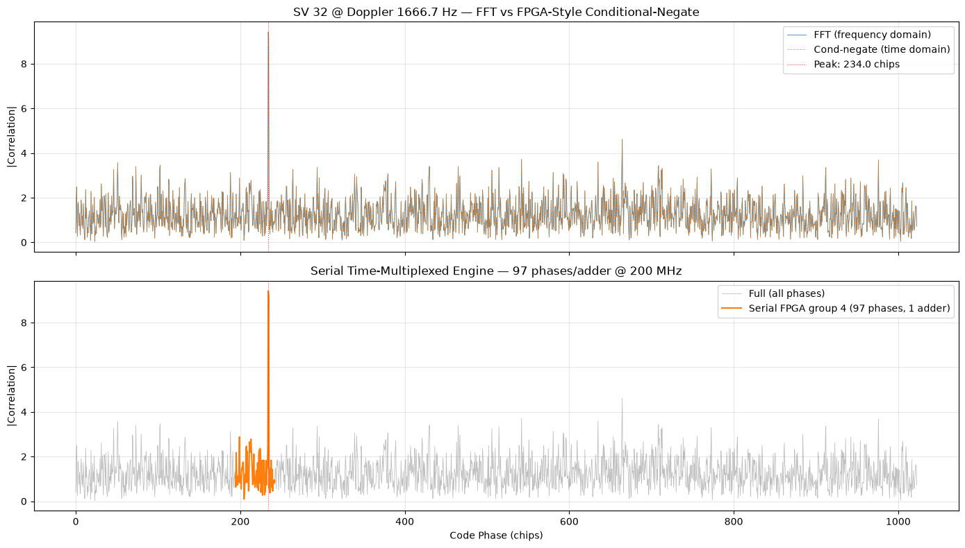
Max error vs FFT reference: 2.32e-15 (should be ~machine epsilon × N) FPGA Architecture @ f_clk = 200 MHz, f_s = 2.046 MHz: Clocks per sample (M): 97 Phases per add/sub unit: 97 Add/sub units for all 2046 phases: 22 Full search time: 22 PRN periods (22 ms) DSP slices required: 0 Serial model (group 4, phases 388-484): Peak phase: 234.0 chips (expected: 234.0) Peak corr: 9.4 (expected: 9.4) Match: True

png

Software Binary Correlator: 1-Bit XOR + Popcount

The FPGA correlator above kept full sample precision but eliminated the multiply via conditional negate. In software we can push the same idea one step further by also quantizing the input to 1 bit per axis (sign bit only). Once both operands are binary, the per-sample multiply collapses to an XOR (sign-disagreement detector) and the length- $N$ accumulation collapses to a popcount (count of mismatches):

Quantity	Bipolar form	Bit form
Sample sign	$s \in \{+1, -1\}$	$\bar{s} \in \{0, 1\}$
Code chip	$c \in \{+1, -1\}$	$\bar{c} \in \{0, 1\}$
Per-sample product	$s \cdot c$	$1 - 2\,(\bar{s} \oplus \bar{c})$
Length- $N$ correlation	$\sum_{k=0}^{N-1} s_k c_k$	$N - 2\,\text{popcount}(\bar{s} \oplus \bar{c})$

For complex baseband, treat $I$ and $Q$ as two independent 1-bit channels and combine the magnitudes:

|R[\phi]| = \sqrt{(N - 2\,\text{popcount}(\bar{I}_\phi \oplus \bar{c}))^2 + (N - 2\,\text{popcount}(\bar{Q}_\phi \oplus \bar{c}))^2}

Per phase hypothesis, this is one XOR (vpxor on x86, EOR on ARM NEON) and one popcount (VPOPCNTQ/POPCNT on x86, CNT on ARM) per 64-bit word — up to 64 input samples retired per instruction on a wide SIMD core, with no multiplies and no floating-point at all. The trade-offs:

Carrier wipeoff still happens at higher precision before quantizing. Once the signal is binary you can no longer rotate the constellation, so Doppler search is unchanged from the methods above.
~1.96 dB SNR loss from hard-limiting Gaussian noise: the well-known $2/\pi$ Van Vleck factor (Jenet & Anderson, 1998). Acceptable for acquisition (a few-dB margin is typically available); tracking loops normally retain more bits.
Code ROM and accumulators shrink dramatically — for GPS C/A at 2 sps, one PRN period is 2046 bits = 256 bytes, easily fitting in L1 cache for thousands of phase hypotheses.

# === Software Binary Correlator: XOR + Popcount on 1-Bit Quantized Samples ===
# Same circular cross-correlation as the FPGA cell above, but every per-sample
# multiply is replaced by a 1-bit XOR and the accumulator by a popcount.
# Theoretical correlation loss vs full precision: 2/pi  (~1.96 dB, Van Vleck).

sv_num = 32
prn_code_bin = generate_ca_code(sv_num)
prn_up_bin   = np.repeat(prn_code_bin, sps)  # {+1, -1}
N = num_corr

# --- Step 1: 1-bit sign quantization on I, Q, and the PRN code ---
# Convention (both signal and code): +sign -> bit 1, -sign -> bit 0
#   XOR == 0 means signs agree (per-sample bipolar product = +1)
#   XOR == 1 means signs disagree (per-sample bipolar product = -1)
# So a length-N correlation in bipolar units is:  N - 2 * popcount(XOR)
I_bin   = (wiped_signal_ref.real >= 0).astype(np.uint8)  # {0, 1}
Q_bin   = (wiped_signal_ref.imag >= 0).astype(np.uint8)
prn_bin = (prn_up_bin > 0).astype(np.uint8)

# --- Step 2: Sliding correlation in clearest-possible 0/1 array form ---
# (popcount on a 0/1 uint8 array is just .sum() — one SIMD reduction)
I_tiled = np.tile(I_bin, 2)
Q_tiled = np.tile(Q_bin, 2)
corr_bin_mag = np.empty(N)
for phi in range(N):
    pc_I = int((I_tiled[phi:phi+N] ^ prn_bin).sum())
    pc_Q = int((Q_tiled[phi:phi+N] ^ prn_bin).sum())
    corr_I = N - 2 * pc_I
    corr_Q = N - 2 * pc_Q
    corr_bin_mag[phi] = np.hypot(corr_I, corr_Q)

# --- Step 3: Same kernel using packed bytes + a real POPCNT ---
# In production, pack 8 bits/byte (or 64 bits/uint64) so a single vectorized
# XOR + bitwise_count covers 8-64 samples per instruction.
def hamming_packed(a_bits, b_bits):
    """popcount(a XOR b) via bit-packed bytes — uses the CPU's POPCNT / CNT."""
    a_pad = np.concatenate([a_bits, np.zeros((-len(a_bits)) % 8, dtype=np.uint8)])
    b_pad = np.concatenate([b_bits, np.zeros((-len(b_bits)) % 8, dtype=np.uint8)])
    xored = np.bitwise_xor(np.packbits(a_pad), np.packbits(b_pad))
    if hasattr(np, "bitwise_count"):
        return int(np.bitwise_count(xored).sum())
    lut = np.array([bin(b).count("1") for b in range(256)], dtype=np.uint16)
    return int(lut[xored].sum())

phi_peak  = int(np.argmax(corr_bin_mag))
pc_packed = hamming_packed(I_tiled[phi_peak:phi_peak+N], prn_bin)
pc_naive  = int((I_tiled[phi_peak:phi_peak+N] ^ prn_bin).sum())
print(f"Packed XOR+popcount matches naive sum at peak: "
      f"{pc_packed == pc_naive}  ({pc_packed} mismatches)")

# --- Step 4: Verify the binary correlator still acquires SV 32 ---
peak_phi_bin   = int(np.argmax(corr_bin_mag))
peak_corr_bin  = corr_bin_mag[peak_phi_bin]
peak_phi_full  = int(np.argmax(np.abs(corr_cond_negate)))
peak_corr_full = np.abs(corr_cond_negate[peak_phi_full])
sample_offset  = peak_phi_bin - peak_phi_full

print(f"\nFloat32 cond-negate : phase = {peak_phi_full/sps:7.2f} chips, |corr| = {peak_corr_full:8.1f}")
print(f"1-bit XOR / popcount: phase = {peak_phi_bin /sps:7.2f} chips, |corr| = {peak_corr_bin :8.1f}")
print(f"Sub-chip offset between estimates: {sample_offset/sps:+.2f} chips "
      f"({sample_offset:+d} sample{'s' if abs(sample_offset)!=1 else ''}) "
      f"-- handed off to the tracking loop below")

# --- Step 5: Empirical quantization loss vs Van Vleck (10*log10(pi/2) ~ 1.96 dB) ---
def peak_to_floor_db(c, idx, exclude=20):
    floor = c.copy().astype(float)
    lo, hi = max(0, idx - exclude), min(len(c), idx + exclude + 1)
    floor[lo:hi] = 0.0
    return 20.0 * np.log10(c[idx] / np.median(floor[floor > 0]))

snr_full = peak_to_floor_db(np.abs(corr_cond_negate), peak_phi_full)
snr_bin  = peak_to_floor_db(corr_bin_mag,             peak_phi_bin)
print(f"\nPeak-to-median-floor SNR (full)  : {snr_full:5.2f} dB")
print(f"Peak-to-median-floor SNR (1-bit) : {snr_bin :5.2f} dB")
print(f"Empirical 1-bit loss             : {snr_full - snr_bin:5.2f} dB"
      f"   (Van Vleck theory: {10*np.log10(np.pi/2):.2f} dB)")

# --- Plot float vs 1-bit correlator overlaid ---
fig, ax = plt.subplots(1, 1, figsize=(14, 4.5))
chips = np.arange(N) / sps
ax.plot(chips, np.abs(corr_cond_negate) / np.abs(corr_cond_negate).max(),
        linewidth=0.7, alpha=0.85, label='Float32 (FPGA cond-negate)')
ax.plot(chips, corr_bin_mag / corr_bin_mag.max(),
        linewidth=0.7, alpha=0.85, label='1-bit XOR + popcount')
ax.axvline(peak_phi_full / sps, color='red', linewidth=0.8, linestyle=':', alpha=0.6,
           label=f'Peak: {peak_phi_full/sps:.1f} chips')
ax.set_xlabel('Code Phase (chips)')
ax.set_ylabel('Normalized |Correlation|')
ax.set_title(f'SV {sv_num} @ Doppler {peak_doppler_hz_ref:.1f} Hz — '
             f'Float32 vs 1-bit Binary Correlator')
ax.legend(loc='upper right')
ax.grid(True, alpha=0.3)
plt.tight_layout()
plt.show()

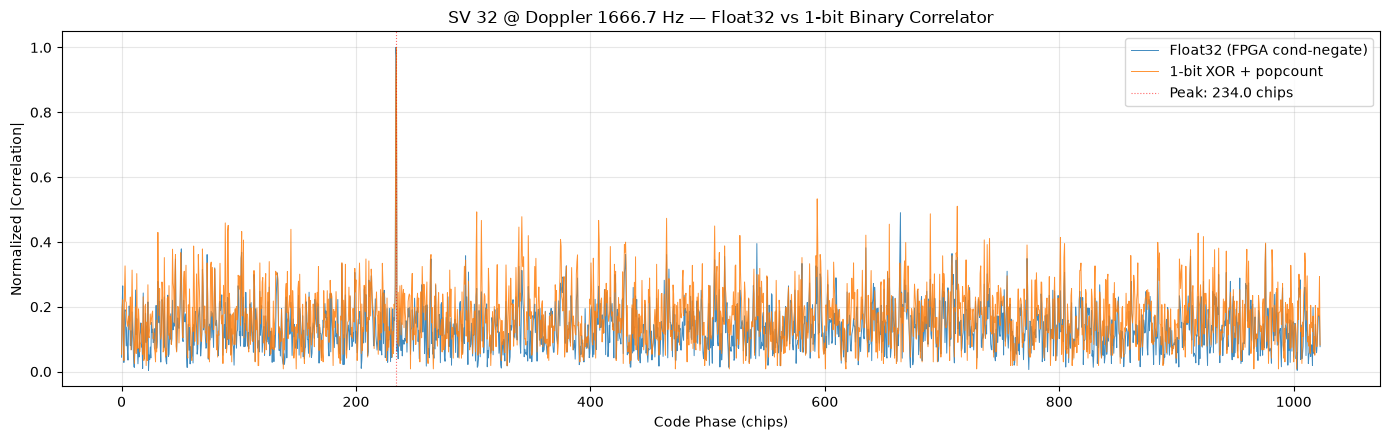
Packed XOR+popcount matches naive sum at peak: True (1188 mismatches) Float32 cond-negate : phase = 234.00 chips, |corr| = 9.4 1-bit XOR / popcount: phase = 234.50 chips, |corr| = 340.0 Sub-chip offset between estimates: +0.50 chips (+1 sample) -- handed off to the tracking loop below Peak-to-median-floor SNR (full) : 18.10 dB Peak-to-median-floor SNR (1-bit) : 15.93 dB Empirical 1-bit loss : 2.17 dB (Van Vleck theory: 1.96 dB)

png

Acquisition to Tracking Handoff

Acquisition produces two coarse parameter estimates that seed the tracking loops rather than feed the demodulator directly:

Acquisition output	Seeds	Why coarse
Doppler estimate $\hat{f}_d$	Carrier NCO / Costas PLL	Accurate only to the acquisition search grid. The PCPS search above used $\approx 101$ Hz steps, so its seed lands within $\pm 50$ Hz of true Doppler. The FFT-native methods (double-buffered, PMF-FFT) quantize to $\Delta f = f_s/N = 1$ kHz bins ( $\pm 500$ Hz residual) — beyond a tracking PLL’s pull-in range, so receivers seeding from those first refine the frequency (a fine-frequency search, or an FLL-assisted PLL whose cross-product frequency discriminator tolerates large offsets) before handing off.
Code-phase estimate $\hat{\tau}$	Code-phase pointer / DLL	Quantized to one input sample — a half chip at 2 samples/chip, i.e. up to $\pm 0.25$ chip of error. Sub-sample alignment must be refined later.

Two parallel loops then close the residual errors and demodulate the data:

Carrier tracking (Costas PLL). A numerically-controlled oscillator (NCO) seeded at $\hat{f}_d$ wipes the residual carrier off each input sample. Once per coherent integration period (1 ms = one PRN period for GPS C/A), the prompt correlator sums $\sum_{n} r[n]\,e^{-j\theta[n]}\,c_\text{local}[n]$ , producing one complex symbol $P = I + jQ$ . For BPSK, the data sign creates a $180°$ ambiguity that a regular PLL would lock on randomly, so we use a Costas phase detector that is invariant to the data sign:

e_\phi = \operatorname{atan2}\bigl(Q \cdot \operatorname{sign}(I),\ |I|\bigr) \approx \theta_\text{err} \quad \text{[rad]}

A second-order PI loop filter integrates $e_\phi$ to drive a frequency correction. By GNSS convention the loop is specified by its noise bandwidth $B_n = \frac{\omega_n}{2}\left(\zeta + \frac{1}{4\zeta}\right)$ , i.e. $\omega_n = 8 \zeta B_n / (1 + 4\zeta^2)$ , with $B_n \approx 15{-}25$ Hz typical for GPS L1 C/A carrier tracking. A loop that narrow cannot pull in the leftover Doppler quickly — its lock-in range is only $\approx 2\zeta\omega_n / 2\pi$ Hz — so software receivers gear-shift: open with a wide pull-in bandwidth, then narrow it once phase lock is achieved. The cell below runs $B_n = 100$ Hz for the first 50 ms (lock-in range $\approx 42$ Hz, comfortably covering the $\leq 50$ Hz seed residual), then shifts to $B_n = 20$ Hz for tracking.

Code tracking — carrier-aided here, DLL in production. Code Doppler is locked to carrier Doppler by the chip-rate-to-carrier-frequency ratio: $f_\text{code} = \hat{f}_d \cdot \frac{1.023\,\text{MHz}}{1575.42\,\text{MHz}} = \hat{f}_d / 1540$ — up to $\pm 3.2$ chips/s over the $\pm 5$ kHz search span, and $\approx 1.1$ chips/s for this SV. Ignoring it would accumulate $\approx 0.22$ chips of misalignment ( $\approx 2$ dB of prompt loss) over the 200 ms window below. The cell therefore carrier-aids the code phase exactly as software receivers do: a fractional sample pointer advances by $f_s / \bigl[ f_\text{PRN} (1 + \hat{f}_d / f_{L1}) \bigr]$ samples per PRN period, and integer sample slips fall out of the rounding automatically. A production receiver adds early and late correlators a half-chip either side of prompt, with an early-minus-late power discriminator driving a code NCO, to track the residual sub-sample errors that carrier aiding cannot see (receiver clock drift, multipath).

After lock, the prompt correlator output rails to $\pm A$ on the $I$ axis with $Q \approx 0$ , and the sign of $I$ recovers the 50 Hz navigation data bits (each bit spans 20 PRN periods — the cell below makes this visible directly, and checks that every bit transition lands on a consistent 20 ms boundary).

Handoff parameters used in the cell below:

Carrier NCO seed: peak_doppler_hz_ref $\approx +1666.7$ Hz (from the PCPS search, $\approx 101$ Hz grid)
Code-phase pointer seed: peak_phi_full (input-sample index from the time-domain conditional-negate correlator)
Coherent integration: $T_\text{coh} = 1$ ms (one PRN period)
Costas loop: optimally damped ( $\zeta = 1/\sqrt{2}$ , the standard choice — critical damping would be $\zeta = 1$ ), noise bandwidth gear-shifted $B_n = 100 \rightarrow 20$ Hz at 50 ms, PI gains from the standard 2nd-order analog prototype.

# === Tracking & BPSK demodulation seeded from the acquisition handoff ===
# Carrier NCO + Costas PLL with explicit Hz/rad units, fed by the prompt
# correlator output. Code phase is carrier-aided: a fractional sample pointer
# advances at the Doppler-corrected code rate, so no DLL is needed over this
# window (a production receiver adds early/late correlators on top).

# --- Handoff state from the previous acquisition cells ---
f_carrier_seed = peak_doppler_hz_ref       # Hz, from the PCPS search (~101 Hz grid)
phi_code_seed  = peak_phi_full             # input-sample offset of prompt window
print(f"Handoff -> Doppler: {f_carrier_seed:+.1f} Hz | "
      f"code phase: {phi_code_seed/sps:.1f} chips ({phi_code_seed} samples)")

# --- Tracking window: 200 ms = 200 PRN periods = 10 nav bits ---
T_track   = 0.20
K         = int(T_track * prn_rate)
N_per_prn = num_corr                       # 2046 samples / 1 ms
T_sym     = 1.0 / prn_rate

# Local upsampled PRN code (±1), aligned to the acquired phase by the read pointer
prn_local = prn_up_hw.astype(np.float64)

# --- Costas PI loop: specified by noise bandwidth Bn (GNSS convention) and
#     gear-shifted from a wide pull-in loop to a narrow tracking loop ---
zeta = 1.0 / np.sqrt(2.0)                  # optimal damping (critical would be 1.0)

def costas_gains(bn_hz):
    """PI gains (Hz of correction per rad of phase error) for a second-order
    loop of noise bandwidth Bn: wn = 8*zeta*Bn / (1 + 4*zeta^2)."""
    wn = 8.0 * zeta * bn_hz / (1.0 + 4.0 * zeta**2)
    return (2.0 * zeta * wn) / (2.0 * np.pi), (wn * wn * T_sym) / (2.0 * np.pi)

bn_pull, bn_track = 100.0, 20.0            # Hz: pull-in / tracking bandwidths
k_shift = 50                               # gear-shift symbol index (50 ms)
Kp, Ki  = costas_gains(bn_pull)

# --- Carrier NCO state: integrator pre-seeded at the handoff Doppler ---
freq_acc    = f_carrier_seed
nco_freq_hz = freq_acc
nco_phase   = 0.0
two_pi_dt   = 2.0 * np.pi / fs
n           = np.arange(N_per_prn)         # hoisted: reused for every block

prompt_iq = np.zeros(K, dtype=complex)
freq_log  = np.zeros(K)
err_log   = np.zeros(K)

sample_ptr = float(phi_code_seed)          # fractional, carrier-aided code phase
for k in range(K):
    if k == k_shift:
        Kp, Ki = costas_gains(bn_track)    # gear-shift: narrow the locked loop

    # 1 ms of input samples at the rounded code-phase pointer (wrap if needed)
    start = int(round(sample_ptr)) % len(iq_in)
    end = start + N_per_prn
    if end <= len(iq_in):
        chunk = iq_in[start:end]
    else:
        chunk = np.concatenate([iq_in[start:], iq_in[:end - len(iq_in)]])

    # --- Carrier wipeoff with the loop NCO ---
    nco_phasor = np.exp(-1j * (nco_phase + two_pi_dt * nco_freq_hz * n))
    wiped = chunk * nco_phasor
    nco_phase = (nco_phase + two_pi_dt * nco_freq_hz * N_per_prn) % (2.0 * np.pi)

    # --- Despread + coherent dump => one prompt symbol ---
    prompt = np.sum(wiped * prn_local)
    prompt_iq[k] = prompt

    # --- BPSK Costas PED: phase error in radians, data-sign removed ---
    err_rad = np.arctan2(prompt.imag * np.sign(prompt.real), abs(prompt.real))
    err_log[k] = err_rad

    # --- PI loop filter -> next NCO frequency ---
    freq_acc   += Ki * err_rad
    nco_freq_hz = freq_acc + Kp * err_rad
    freq_log[k] = nco_freq_hz

    # --- Carrier-aided code advance: the received PRN period spans
    #     fs / (prn_rate*(1 + fd/fL1)) samples, not exactly N_per_prn ---
    sample_ptr = (sample_ptr + fs / (prn_rate * (1.0 + nco_freq_hz / fc_l1))) % len(iq_in)

# --- Pull out the 50 Hz navigation bit stream from sign(I) ---
nav_bits_per_prn = np.sign(prompt_iq.real).astype(int)

# Post-lock metrics only (k >= k_shift): the pull-in transient is excluded
i_q_db = 20.0 * np.log10(np.mean(np.abs(prompt_iq.real[k_shift:])) /
                         np.mean(np.abs(prompt_iq.imag[k_shift:])))
print(f"\nLoop final freq:    {freq_log[-1]:+.2f} Hz "
      f"(pulled {freq_log[-1]-f_carrier_seed:+.2f} Hz from handoff)")
print(f"Post-lock |I|/|Q|:  {i_q_db:5.2f} dB  -> clean BPSK lock")

trans_idx = np.flatnonzero(np.diff(nav_bits_per_prn[k_shift:]) != 0) + k_shift + 1
print(f"Nav-bit transitions after lock: {len(trans_idx)}  (each bit = 20 PRN periods)")
if len(trans_idx):
    print(f"Bit-edge check: transitions land at PRN index mod 20 = "
          f"{sorted(set(int(t) % 20 for t in trans_idx))}  "
          f"(a single value -> consistent 20 ms bit boundaries)")

# --- Convergence diagnostics ---
fig, axs = plt.subplots(3, 1, figsize=(13, 8), sharex=True)
axs[0].plot(freq_log, linewidth=0.9)
axs[0].axhline(f_carrier_seed, color='gray', linestyle=':',
               label=f'Acquisition handoff: {f_carrier_seed:.1f} Hz')
axs[0].axvline(k_shift, color='C3', linestyle='--', linewidth=1,
               label=f'Gear shift: Bn = {bn_pull:.0f} -> {bn_track:.0f} Hz')
axs[0].set_ylabel('NCO freq (Hz)')
axs[0].set_title('Costas PLL pull-in from acquisition handoff')
axs[0].legend(loc='lower right'); axs[0].grid(alpha=0.3)

axs[1].plot(prompt_iq.real, linewidth=0.7, label='I (data bit × A)')
axs[1].plot(prompt_iq.imag, linewidth=0.7, label='Q (phase error)', alpha=0.8)
axs[1].set_ylabel('Prompt correlator')
axs[1].legend(loc='upper right'); axs[1].grid(alpha=0.3)

axs[2].plot(err_log, linewidth=0.7)
axs[2].set_ylabel('Costas phase err (rad)')
axs[2].set_xlabel('PRN period (ms)')
axs[2].grid(alpha=0.3)

plt.tight_layout(); plt.show()

# Post-lock BPSK constellation (pull-in transient excluded)
plot.IQ(prompt_iq[k_shift:], title=f'Despread BPSK constellation — SV {sv_num} '
                      f'(post-lock, |I|/|Q| = {i_q_db:.1f} dB)', alpha=0.4)
plt.show()

Handoff -> Doppler: +1666.7 Hz | code phase: 234.0 chips (468 samples)

Loop final freq: +1697.45 Hz (pulled +30.78 Hz from handoff) Post-lock |I|/|Q|: 21.23 dB -> clean BPSK lock Nav-bit transitions after lock: 4 (each bit = 20 PRN periods) Bit-edge check: transitions land at PRN index mod 20 = [9] (a single value -> consistent 20 ms bit boundaries)

png

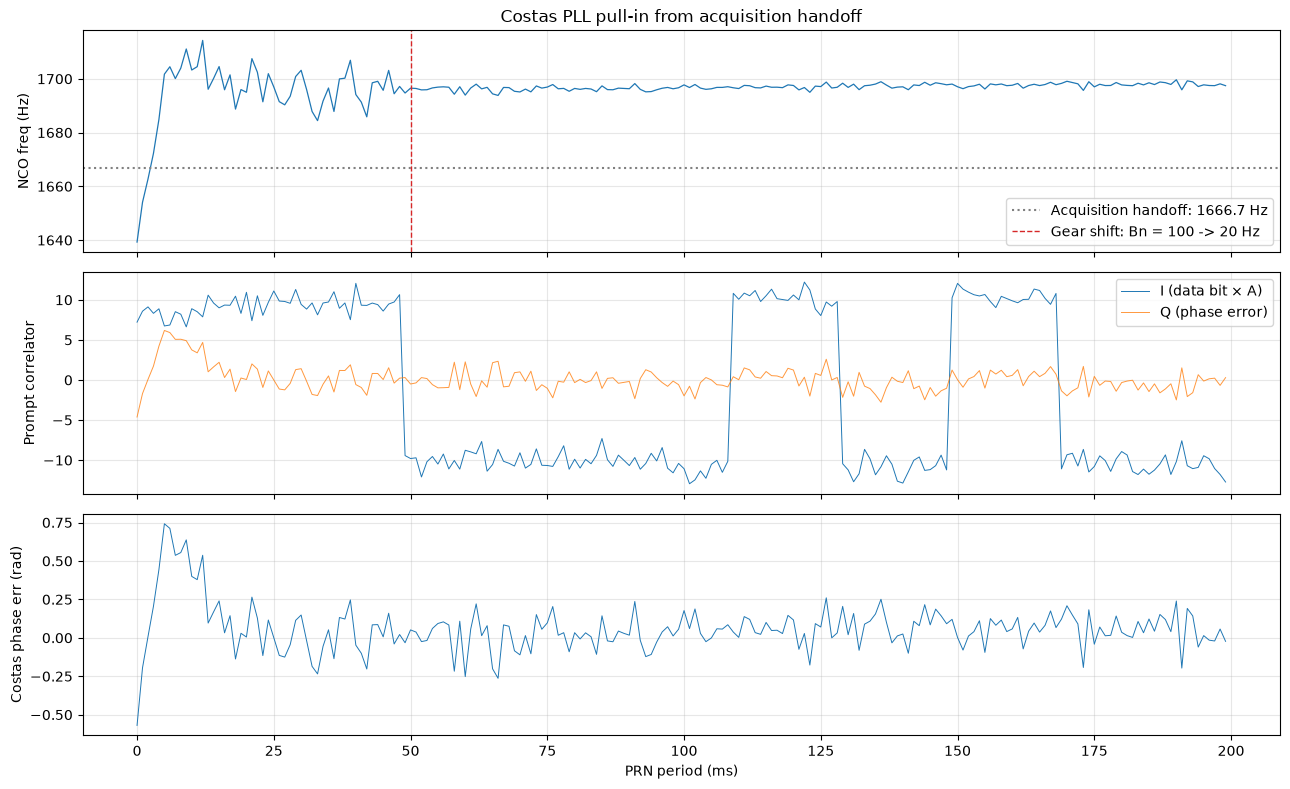
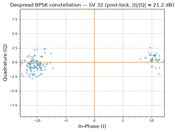
GPS References

GPS Signals - Wikipedia
Building a GPS Receiver - Phillip Tennen: great blog and software source (gypsum) on making a GPS receiver from a simple RTL-SDR.
Building a GPS Receiver from Scratch - YouTube Series with associated GitHub repo (chrisdoble/gps-receiver)
Questions about FFT Based GPS Acquisition - DSP Stack Exchange
- Joint Frequency and Delay Correlation - Matlab File Exchange - Dan Boschen
GPS (GNSS) signal processing chain from a received raw signal, signal acquisition, tracking to demodulation: An introduction
GNSS-SDR: An open-source Global Navigation Satellite Systems software-defined receiver.
GPS Receiver Acquisition and Tracking Using C/A-Code
Timing SDR recordings with GPS
GPS disciplined oscillator - Wikipedia
osqzss/gps-sdr-sim: software-defined GPS Signal Simulator.
- Mictronics/pluto-gps-sim
JiaoXianjun/GNSS-GPS-SDR: some efforts on GPS replay, receive and test.
GPS Real Time Kinematics (RTK)- Sparkfun
GPS Beamforming with Low-cost RTL-SDRs- GRCon17
GPS - Bartosz Ciechanowski
Homemade GPS Receiver - Andrew Holme

Other Methods of PNT

Signal Structure of the Starlink Ku-Band Downlink and Timing Properties of the Starlink Ku-Band Downlink: Abstract—We develop a technique for blind signal identification of the Starlink downlink signal in the 10.7 to 12.7 GHz band and present a detailed picture of the signal’s structure. Importantly, the signal characterization offered herein includes the exact values of synchronization sequences embedded in the signal that can be exploited to produce pseudorange measurements. Such an understanding of the signal is essential to emerging efforts that seek to dual-purpose Starlink signals for positioning, navigation, and timing, despite their being designed solely for broadband Internet provision.
- Also Unveiling Starlink for PNT, Starlink for PNT: A Trick or a Treat? and Acquisition and Tracking of Starlink LEO Satellite Signals in Low SNR Regime by OSU
- https://radionavlab.ae.utexas.edu/publications/ has interesting research on PNT and distributed array effects.
Multi-Constellation Blind Beacon Estimation, Doppler Tracking, and Opportunistic Positioning with OneWeb, Starlink, Iridium NEXT, and Orbcomm LEO Satellites
Unveiling Starlink LEO Satellite OFDM-Like Signal Structure Enabling Precise Positioning
Receiver Design for Doppler Positioning with Leo Satellites
CCSDS Data Transmission and PN Ranging for 2 GHz CDMA Link via Data Relay Satellite

Known Terrestrial Signals

LTE Disciplined Oscillator