RF Impairments & Corrections

Est. read time: 2 minutes | Last updated: June 16, 2026 by John Gentile

Contents

Overview
Additive Noise
- Thermal Noise
I/Q Offset Correction
DC Offset / LO Leakage
- DC Nulling Filter
Wireless Channels
References

from IPython.display import YouTubeVideo, Markdown
import inspect

import numpy as np
import matplotlib.pyplot as plt
import scipy
from rfproto import filter, impairments, plot, sig_gen

Overview

Below is a quick reference of common RF impairments encountered in digital communications systems. For each, $x$ is the ideal transmitted symbol and $y$ is what we observe at the slicer.

Impairment	Model (received $y$ )	I/Q constellation signature
AWGN (additive white Gaussian noise)	$y = x + n,\ \ n \sim \mathcal{CN}(0,\sigma^2)$	Each ideal symbol turns into a round, fuzzy cloud of the same size. Every symbol is equally blurred; the cloud just grows as SNR drops.
LO phase noise	$y = x \cdot e^{j\phi(t)},\ \ \phi(t)$ a Wiener (random‑walk) process	Symbols get smeared along an arc (tangent to a circle centered on the origin), because a random phase rotates them about $0$ . Outer symbols smear farther in absolute distance since arc length scales with $\lvert x\rvert$ .
Carrier frequency offset (CFO)	$y_n = x_n \cdot e^{j 2\pi \Delta f\, n T_s}$	The entire constellation spins as a rigid body at rate $\Delta f$ . Left uncorrected over many symbols, the points trace concentric rings.
I/Q gain imbalance	$y = (1+\varepsilon)\,x_I + j(1-\varepsilon)\,x_Q$	The I and Q axes are scaled by different amounts, so a square constellation (e.g., QPSK) becomes a rectangle — an axis‑aligned stretch/squash.
I/Q phase imbalance	$y = x_I + j\bigl(x_I\sin\psi + x_Q\cos\psi\bigr)$	The I and Q channels are no longer exactly 90° apart, so the constellation gets sheared: a square becomes a parallelogram.
PA compression (AM/AM + AM/PM)	$\lvert y\rvert = g(\lvert x\rvert)$ saturating; $\angle y = \angle x + \theta(\lvert x\rvert)$	Outer (high‑power) symbols are pulled inward and twisted in phase by the amplifier’s nonlinearity. Inner symbols are roughly untouched, so the outline of the constellation looks “pinched.”
Timing residual (wrong sample instant)	$y_n = \sum_k x_k\,h\bigl((n-k)T_s + \tau\bigr)$	We sample off the eye’s center, so neighboring symbols leak in (ISI). Each ideal point splits into several data‑dependent “satellite” clusters, and the eye diagram closes.
Sample‑rate / clock drift	$\tau(n) = \tau_0 + \Delta\!\cdot\!n$ (timing offset accumulates)	Same ISI mechanism as above, but the timing error grows linearly with sample index, so the smear gets progressively worse over the burst.
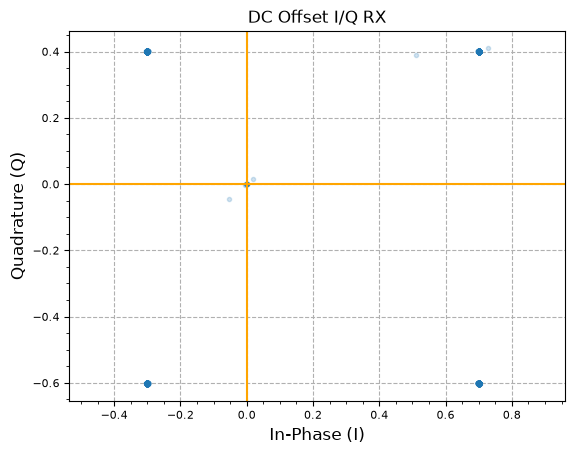
DC offset / LO leakage	$y = x + c,\ \ c \in \mathbb{C}$ constant	The whole constellation is rigidly translated off the origin by the constant $c$ (a bright spot also appears at DC in the spectrum).

num_symbols = 2048
baud = 1e6
rand_symbols = np.random.randint(0, 4, num_symbols)
L = 2
fs = L * baud
rolloff = 0.35
num_filt_symbols = 12

x = sig_gen.gen_mod_signal(
    "QPSK",
    rand_symbols,
    fs,
    baud,
    "RRC",
    rolloff,
    num_filt_symbols,
)

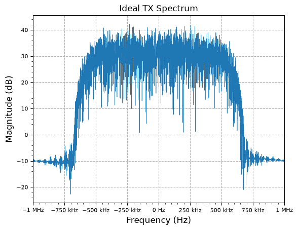
plot.spec_an(x, fs=fs, fft_shift=True, show_SFDR=False, y_unit="dB", title="Ideal TX Spectrum")
plt.show()

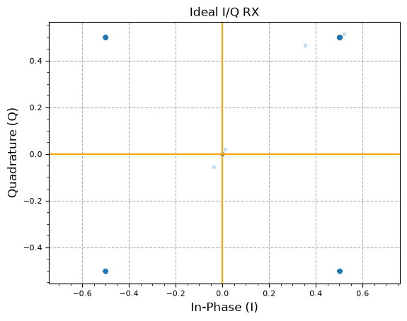
# Show ideal QPSK at receiver w/matched RRC filter
rrc_coef = filter.RootRaisedCosine(L * baud, baud, rolloff, 2 * num_filt_symbols * L + 1)
y_ideal = scipy.signal.lfilter(rrc_coef, 1, x)
plot.IQ(y_ideal[::2], alpha=0.2, title="Ideal I/Q RX")
plt.show()

png

YouTubeVideo('PNMOwhEHE6w')

YouTubeVideo('LBLvmNyAdSI')

Additive Noise

Thermal Noise

Defined by the equation:

N = kTBF_{N}

Where:

$k$ is the Boltzmann Constant
$T$ is the device temperature in Kelvin
$B$ is the receiver bandwidth in Hertz
$F_{N}$ is the noise factor of the system

Markdown(f"```python\n{inspect.getsource(impairments.thermal_noise)}\n```")

def thermal_noise(T, B, Fn):
    return scipy.constants.k * T * B * Fn

At room temp (290 Kelvin), this relates to a noise power spectral density of -144 dBW/MHz, which means for every 1 MHz of bandwidth, -144 dBW of thermal noise is added).

room_temp = 290
bw = 10e6
# convert to dBW, then +30 to dBmW
therm_noise = 10*np.log10(impairments.thermal_noise(room_temp, bw, 1)) + 30
print(f"Thermal noise at room temp, {bw/1e6}MHz bandwidth: {therm_noise:.4} dBmW")

Thermal noise at room temp, 10.0MHz bandwidth: -104.0 dBmW

I/Q Offset Correction

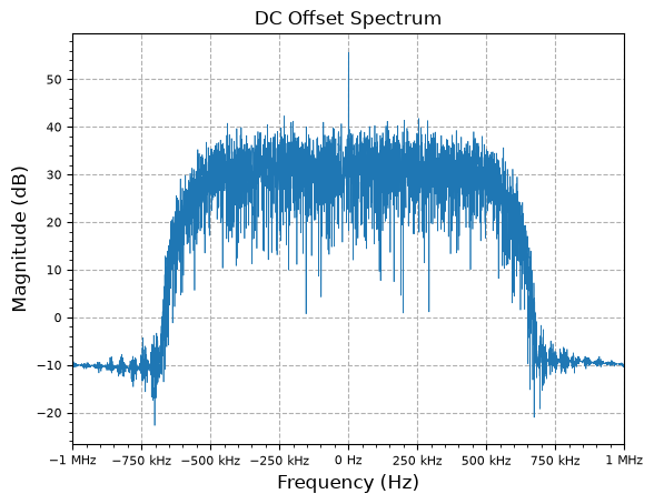
DC Offset / LO Leakage

x_dc_offset = x + 0.2 - 1j*0.1
plot.spec_an(x_dc_offset, fs=fs, fft_shift=True, show_SFDR=False, y_unit="dB", title="DC Offset Spectrum")
plt.show()

y_dc_offset = scipy.signal.lfilter(rrc_coef, 1, x_dc_offset)
plot.IQ(y_dc_offset[::2], alpha=0.2, title="DC Offset I/Q RX")
plt.show()

png

DC Nulling Filter

Since the offset is just a constant (i.e., a tone at $f = 0$ ), all we need is a high‑pass filter with a sharp notch at DC and (close to) unity gain everywhere else. The classic single‑pole “DC blocker” (e.x. in Xilinx WP279) does exactly this with one multiplier and two adds per sample:

y_\text{out}[n] \;=\; y[n] \;-\; y[n-1] \;+\; \alpha\, y_\text{out}[n-1]

which has the transfer function

H(z) \;=\; \frac{1 - z^{-1}}{1 - \alpha\, z^{-1}}.

This works because of where its pole and zero sit on the $z$ ‑plane:

Zero at $z = 1$ (i.e., $\omega = 0$ ): the numerator $1 - z^{-1}$ vanishes at DC, so $H(e^{j0}) = 0$ . Any constant offset is killed exactly.
Pole at $z = \alpha$ , just inside the unit circle (typically $\alpha \in [0.99,\ 0.9999]$ ): the denominator nearly cancels the zero everywhere except very close to DC, pulling $\lvert H(e^{j\omega}) \rvert$ back up to ~1 over the rest of the band.

The result is a narrow notch at DC that leaves the signal band essentially untouched. The trade‑off is set by $\alpha$ :

$\alpha$ closer to 1 → narrower notch (less in‑band distortion), but slower transient settling on startup.
$\alpha$ closer to 0 → wider notch (faster settling), but more low‑frequency signal content is attenuated.

A handy rule‑of‑thumb for the $-3\,\text{dB}$ cutoff is

f_{\text{3dB}} \;\approx\; \frac{1 - \alpha}{2\pi}\, f_s,

so picking $\alpha$ amounts to deciding how much low‑frequency content you’re willing to sacrifice for guaranteed DC rejection.

For fixed-point integer data samples, like in FPGAs, we can go one-step further and perform the multiplication of $\alpha$ as a hardware-friendly, $n$ -bit right-shift and subtract, since right shifting is the same as dividing by $2^N$ . For example for a desired $\alpha = 0.999$ :

\alpha = 1 - \frac{1}{2^{n}} \rightarrow 1 - \frac{1}{2^{10}} \approx 0.999

n = len(x_dc_offset)
y_dc_offset_corrected = np.zeros(n) + 1j*np.zeros(n)

b = 10
z0 = 0.0 + 1j*0.0
z1 = 0.0 + 1j*0.0
for i in range(n):
    y_dc_offset_corrected[i] = z1
    rshft = z1 / (2**b)
    z1 = z1 - rshft + x_dc_offset[i] - z0
    z0 = x_dc_offset[i]

y_dc_offset_corr = scipy.signal.lfilter(rrc_coef, 1, y_dc_offset_corrected)
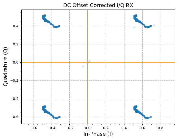
plot.IQ(y_dc_offset_corr[1::2], alpha=0.2, title="DC Offset Corrected I/Q RX")
plt.show()

png

Wireless Channels

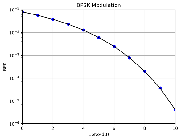
N = 5000000
EbNodB_range = range(11)
itr = len(EbNodB_range)
ber = [None]*itr

for n in range (itr): 
    EbNodB = EbNodB_range[n]   
    EbNo=10.0**(EbNodB/10.0)
    x = 2 * (np.random.rand(N) >= 0.5) - 1
    noise_std = 1/np.sqrt(2*EbNo)
    y = x + noise_std * np.random.randn(N)
    y_d = 2 * (y >= 0) - 1
    errors = (x != y_d).sum()
    ber[n] = 1.0 * errors / N

plt.figure()
plt.plot(EbNodB_range, ber, 'bo', EbNodB_range, ber, 'k')
plt.axis([0, 10, 1e-6, 0.1])
plt.xscale('linear')
plt.yscale('log')
plt.xlabel('EbNo(dB)')
plt.ylabel('BER')
plt.grid(True)
plt.title('BPSK Modulation')
plt.show()

png