Position Navigation and Timing (PNT)
Est. read time: 2 minutes | Last updated: July 06, 2025 by John Gentile
Contents
![]()
import numpy as np
from scipy import signal
import matplotlib.pyplot as plt
from rfproto import plot
GPS
#partial_data = np.fromfile("/Users/jgentile/Downloads/nov_3_time_18_48_st_ives", dtype=np.complex64, count=2*32768, offset=0)
#plot.fft_intensity_plot(partial_data, fft_len=4096, fft_div=16)
#plot.plt.show()
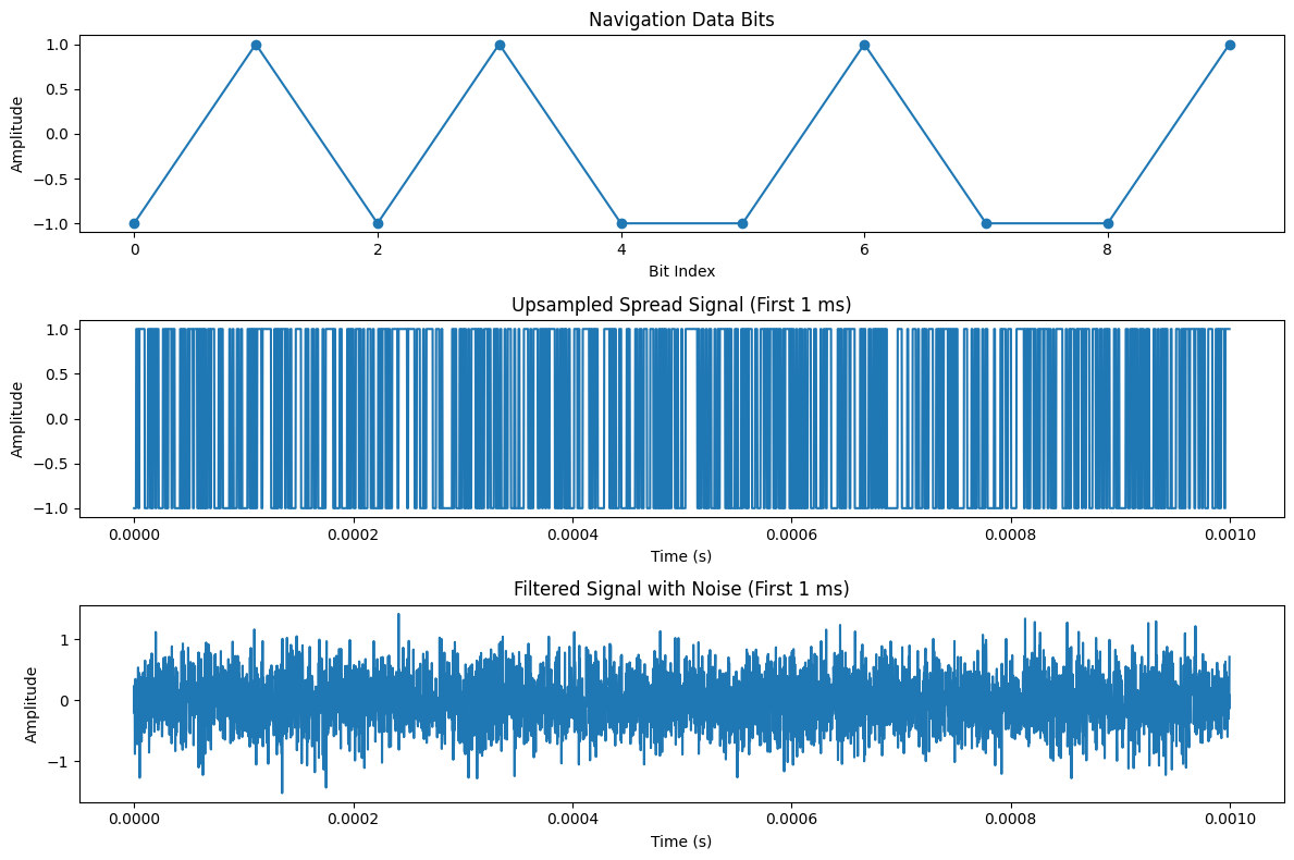
This code:
- Defines GPS L1 C/A signal parameters (chip rate: 1.023 MHz, code length: 1023 chips, bit rate: 50 bps).
- Generates a Gold code for PRN 1 using two LFSRs (G1 and G2) with specific tap settings.
- Creates random navigation data bits and spreads them with the Gold code.
- Upsamples the signal to simulate the chip rate with 16 samples per chip.
- Applies a Butterworth band-pass filter to shape the spectrum (1–2 MHz for simplicity).
- Adds Gaussian noise to emulate typical GPS signal conditions.
- Plots the navigation bits, upsampled spread signal, and noisy filtered signal, saving the result as ‘gps_signal.png’.
The signal is simulated at baseband rather than the actual L1 frequency (1575.42 MHz) to keep computations manageable. The Gold code generation follows the GPS C/A structure, using PRN 1 as an example. The filter and noise parameters are chosen to approximate real GPS signal characteristics.
To extend this:
- Use different PRNs by changing the phase_select taps (refer to GPS ICD-200 for tap settings).
- Modulate onto a carrier for a more complete simulation.
- Adjust noise power or filter parameters for different scenarios.
# Parameters for GPS L1 C/A signal
chip_rate = 1.023e6  # C/A code chip rate (Hz)
code_length = 1023   # Length of C/A Gold code
bit_rate = 50        # Navigation data bit rate (bps)
samples_per_chip = 4  # Upsampling factor
fs = chip_rate * samples_per_chip  # Sampling frequency
bit_duration = 1 / bit_rate  # Duration of one navigation bit
chips_per_bit = int(chip_rate / bit_rate)  # Chips per data bit (20460)

# Generate a Gold code (simplified for one PRN, e.g., PRN 1)
def generate_gold_code(prn=1):
    # LFSR settings for GPS C/A code (G1 and G2 shift registers)
    g1 = np.ones(10, dtype=int)  # G1: x^10 + x^3 + 1
    g2 = np.ones(10, dtype=int)  # G2: x^10 + x^9 + x^8 + x^6 + x^3 + x^2 + 1
    code = np.zeros(code_length, dtype=int)

    # Phase selection for PRN 1 (taps at positions 2 and 6)
    phase_select = [2, 6]  # For PRN 1

    for i in range(code_length):
        code[i] = g1[9] ^ g2[phase_select[0]-1] ^ g2[phase_select[1]-1]
        g1_feedback = g1[9] ^ g1[2]
        g2_feedback = g2[9] ^ g2[8] ^ g2[7] ^ g2[5] ^ g2[2] ^ g2[1]
        g1 = np.roll(g1, 1)
        g2 = np.roll(g2, 1)
        g1[0] = g1_feedback
        g2[0] = g2_feedback

    return 2 * code - 1  # Convert to bipolar (+1, -1)

# Generate navigation data bits
num_bits = 10
nav_bits = np.random.randint(0, 2, num_bits) * 2 - 1  # Bipolar (-1, +1)

# Generate Gold code
gold_code = generate_gold_code(prn=1)

# Spread the navigation data with Gold code
spread_signal = np.array([])
for bit in nav_bits:
    spread_signal = np.append(spread_signal, bit * gold_code)

# Upsample the spread signal
upsampled_signal = np.repeat(spread_signal, samples_per_chip)

# Time vector for the signal
t = np.arange(len(upsampled_signal)) / fs

# Apply band-pass filter to emulate GPS signal bandwidth
f_low = 1e6  # Approximate bandwidth for C/A code
f_high = 2e6
b, a = signal.butter(4, [f_low, f_high], btype='band', fs=fs)
filtered_signal = signal.lfilter(b, a, upsampled_signal)

# Add noise to simulate realistic signal (SNR ~ -20 dB for GPS)
noise_power = 0.1  # Adjusted for typical GPS signal SNR
noise = np.random.normal(0, np.sqrt(noise_power), len(filtered_signal))
noisy_signal = filtered_signal + noise
#noisy_signal = upsampled_signal

len1ms = int(0.001*fs)

# Plot the results
plt.figure(figsize=(12, 8))

plt.subplot(3, 1, 1)
plt.plot(nav_bits, 'o-')
plt.title('Navigation Data Bits')
plt.xlabel('Bit Index')
plt.ylabel('Amplitude')

plt.subplot(3, 1, 2)
plt.plot(t[:len1ms], upsampled_signal[:len1ms])
plt.title('Upsampled Spread Signal (First 1 ms)')
plt.xlabel('Time (s)')
plt.ylabel('Amplitude')

plt.subplot(3, 1, 3)
plt.plot(t[:len1ms], noisy_signal[:len1ms])
plt.title('Filtered Signal with Noise (First 1 ms)')
plt.xlabel('Time (s)')
plt.ylabel('Amplitude')

plt.tight_layout()
plt.show()
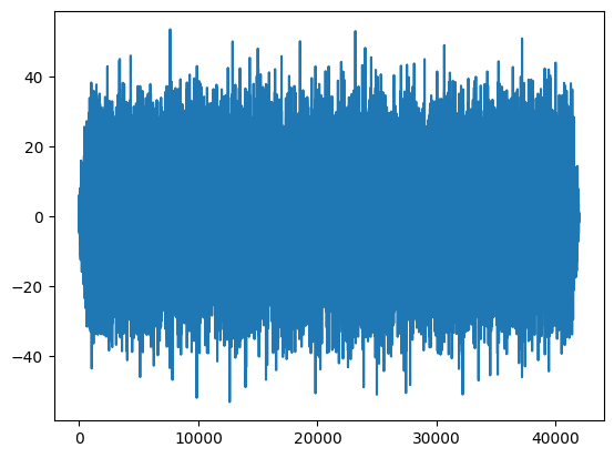
result = np.correlate(noisy_signal,gold_code, mode='full')
plt.plot(result)
plt.show()
# Zero-pad PRN code to match input signal length
prn_code_padded = np.pad(gold_code, (0, len1ms - len(gold_code)), 'constant')
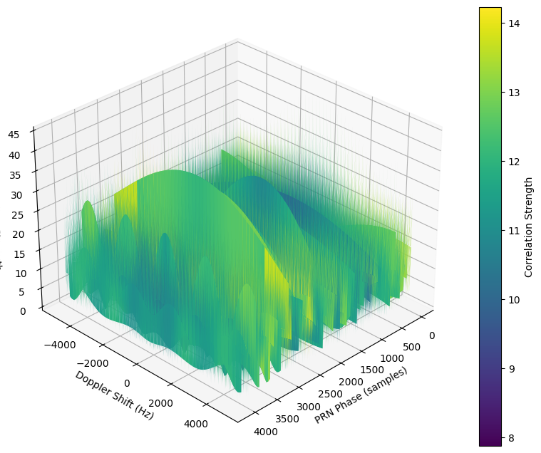
# Define Doppler shift range to search (in Hz)
doppler_shifts = np.linspace(-5000, 5000, 100) # -5 kHz to 5 kHz, 100 steps
# Array to store correlation results: [doppler shifts, time delays]
correlation_results = np.zeros((len(doppler_shifts), len1ms))
for dop_idx, doppler_shift in enumerate(doppler_shifts):
# Time vector for Doppler adjustment
t = np.arange(len1ms) / (2 * fs)
# Apply Doppler shift with complex exponential (phasor)
doppler_adjustment = np.exp(-1j * 2 * np.pi * doppler_shift * t)
adjusted_signal = noisy_signal[:len1ms] * doppler_adjustment
# FFT of adjusted signal and PRN code
fft_signal = np.fft.fft(adjusted_signal)
fft_prn = np.fft.fft(prn_code_padded)
# Frequency domain cross-correlation
cross_corr_freq = fft_signal * np.conj(fft_prn)
cross_corr_time = np.fft.ifft(cross_corr_freq)
# Store magnitude of correlation
correlation_results[dop_idx, :] = np.abs(cross_corr_time)
# Create a new figure for the 3D plot
fig = plt.figure(figsize=(10, 8))
ax = fig.add_subplot(111, projection='3d')
# Define the x and y axes
x = np.arange(len1ms) # PRN phase (time delays in samples)
y = doppler_shifts # Doppler shifts in Hz
X, Y = np.meshgrid(x, y) # Create a 2D grid for plotting
# Correlation strength for this satellite
Z = correlation_results
# Plot the 3D surface
surf = ax.plot_surface(X, Y, Z, cmap='viridis')
# Set axis labels
ax.set_xlabel('PRN Phase (samples)')
ax.set_ylabel('Doppler Shift (Hz)')
ax.set_zlabel('Correlation Strength')
ax.view_init(elev=30, azim=45)
# Add a colorbar to indicate correlation strength
fig.colorbar(surf, label='Correlation Strength')
plt.show()
References
- Building a GPS Receiver - Phillip Tennen: great blog and software source (gypsum) on making a GPS receiver from a simple RTL-SDR.
- Building a GPS Receiver from Scratch - YouTube Series with associated GitHub repo (chrisdoble/gps-receiver)
- GNSS-SDR: An open-source Global Navigation Satellite Systems software-defined receiver.
- GPS Receiver Acquisition and Tracking Using C/A-Code
- GPS disciplined oscillator - Wikipedia
- osqzss/gps-sdr-sim: software-defined GPS Signal Simulator.
- JiaoXianjun/GNSS-GPS-SDR: some efforts on GPS replay, receive and test.
- GPS Real Time Kinematics (RTK)- Sparkfun
- GPS Beamforming with Low-cost RTL-SDRs- GRCon17
- GPS - Bartosz Ciechanowski
Other Methods of PNT
Blind Signal Receiver for PNT
- Signal Structure of the Starlink Ku-Band Downlink: Abstract—We develop a technique for blind signal identification of the Starlink downlink signal in the 10.7 to 12.7 GHz band and present a detailed picture of the signal’s structure. Importantly, the signal characterization offered herein includes the exact values of synchronization sequences embedded in the signal that can be exploited to produce pseudorange measurements. Such an understanding of the signal is essential to emerging efforts that seek to dual-purpose Starlink signals for positioning, navigation, and timing, despite their being designed solely for broadband Internet provision.
- https://radionavlab.ae.utexas.edu/publications/ has interesting research on PNT and distributed array effects.
- Multi-Constellation Blind Beacon Estimation, Doppler Tracking, and Opportunistic Positioning with OneWeb, Starlink, Iridium NEXT, and Orbcomm LEO Satellites
- Unveiling Starlink LEO Satellite OFDM-Like Signal Structure Enabling Precise Positioning
- Receiver Design for Doppler Positioning with Leo Satellites
- CCSDS Data Transmission and PN Ranging for 2 GHz CDMA Link via Data Relay Satellite
Known Terrestrial Signals
Maintained by John Gentile • Found a problem on this site? File an Issue
This work is licensed under a Creative Commons Attribution 4.0 International License.![]()